Welcome to Adaptation Strategies
Mapping Habitat Cores and Assessing Connectivity with GIS

Lesson Topics

This lesson will cover three topics and take approximately 40-50 minutes to complete. We recommend working through each topic in the order in which they are listed below.

Topic 1: Mapping Cores

In this topic

• Define core habitat
• Understand models of habitat as surrogates for species distribution
• Explore techniques to identify, map, and model core habitat

Topic 2: Connectivity

Here you will:

• Understand importance of connectivity
• Use spatial analysis concepts and methods for evaluating habitat connectivity and landscape permeability

Topic 3: Applying Core and Connectivity Tools in GIS

Finally you will:

• Apply techniques to identify, map, and model core habitat
• Apply methods for evaluating habitat connectivity & landscape permeability

This lesson is drawn from Chapters 9 and 10 in Craighead and Convis and from the article by Nikolakaki (2004, pdf). Other papers supplementing this lesson are posted with the Unit readings, including:

Brodie JF, Giordano AJ, Dickson B et al (2015) Evaluating multispecies landscape connectivity in a threatened tropical mammal community. Conservation Biology 29(1):122-132

Freeman RC, Bell KP (2011) Conservation versus cluster subdivisions and implications for habitat connectivity. Landscape and Urban Planning 101(1):30-42

Mapping Cores

In landscape ecology and conservation planning, we use a specific vocabulary to describe the relationships of species to the landscape and the spatial patterns of those relationships. Let’s review some of these terms from the last module:

1. Habitat – sites with appropriate biotic and abiotic features required by a given species. Some species may require different types of habitat for different activities, such as feeding, nesting, or migrating.

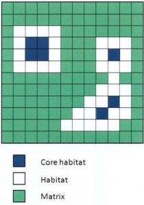
2. Patch – a contiguous region of the same habitat.
3. Connected – habitat occurring as few large patches, arranged in close proximity for dispersal, or within a hospitable matrix or buffer for crossing
4. Fragmented – habitat occurring as many small patches
5. Interior/core area – part of habitat patches not influenced by edge effects
6. Edge/edge effects – the boundary between two habitat types, or changes in ecological factors near patch boundaries.

Defining Core Habitat

The term ‘core habitat‘ is commonly used, but its meaning is contextually dependent.

On the one hand, the word “core” can be defined as the basic or most important part of something. This meaning of core habitat has been used in conservation since 1970’s, when UNESCO’s Man and the Biosphere program included the term ‘core’ in its statutory framework. UNESCO specified that a biosphere reserve includes “a legally constituted core area or areas devoted to long-term protection, according to the conservation objectives of the biosphere reserve, and of sufficient size to meet these objectives” (pg. 219). Using this general definition, core area is often defined in the context of a particular conservation project.

Alternatively, it can be defined ecologically as an interior area free of edge effects, as an area free of human influence, or according to demographics, as an area large enough to support a viable population of a particular species.

Here, we will use a broad definition of core as “an area or patch of relatively intact habitat that is sufficiently large to support more than one individual of a species.”

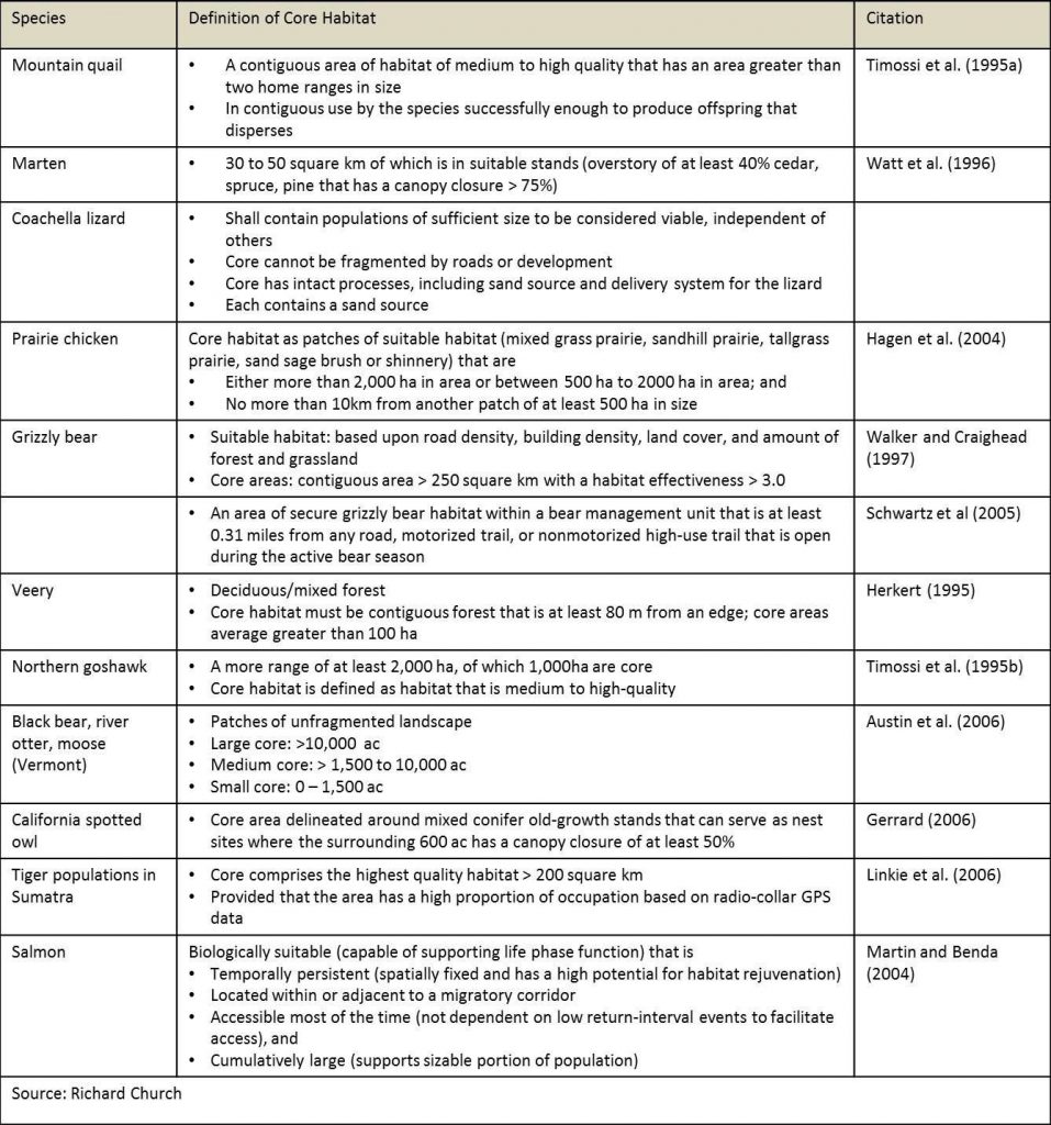
Examples of Core Habitat

Core habitat can be defined based on rules or metrics set by a conservation team or study. In the table below, specific definitions of core habitat are shown for different target species.

Starting point: A map of suitable habitat

The process of identifying core habitat begins with a map of suitable habitat for the species or community in question.

General approaches to mapping suitable habitat include:

• identify the landscape requirements for a given species and map
• species presence mapping
• predictive habitat models
• wildlife habitat relationship models

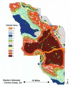
Often, a habitat suitability map classifies the landscape based on an area’s value as habitat for a species of interest – sometimes as simply ‘suitable’ or ‘not suitable’
and other times with ranks or values of suitability.

In the example here, the landscape has been classified according to its habitat value for the kit fox, with areas of high suitability receiving a value of 6 and areas of very low suitability a value of -20.

For many conservation planning applications, the mapped habitat suitability can be used to delineate core habitats as we will explore.

Approaches to determining core habitat

In many conservation applications, a mapped range of habitat values, or habitat threshold, can be used to define core habitat. In this approach, all habitat with a certain value (such as suitable) and in contiguous blocks of some minimum size are considered core habitat.

For example, a project aimed at siting a wildlife preserve might prioritize habitat for endangered species. In this case, conservation practitioners might use the U.S. Fish and Wildlife Service’s Critical Habitat Mapper to locate the habitat of all endangered species in a region of interest. Any areas identified as habitat for an endangered species would then be a core habitat in that preserve.

Here we will look at 5 basic approaches to defining and mapping core areas:

• Buffer defined core
• Density defined core
• Patch defined core
• Population defined core
• Territory separated core

Buffer defined core

Core habitat is defined as suitable habitat that is at least some minimum specified distance (buffer) to any edge. FRAGSTATS or similar tools can be used to calculate core habitat based on some buffer distance.

Density defined core

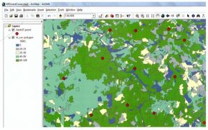
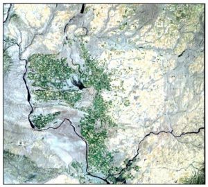
Core habitat is defined by a measurement of some important habitat characteristic. For example, percent canopy coverage is an essential characteristic in determining where California spotted owls nest and forage, with the average canopy closure in a 600 acre radius being the best determinant of suitability for nesting.

From a map of canopy closure, we can generate a map of suitable nesting sites based on average canopy closure using the Focal Statistics tool in ArcGIS – using a circle option to calculate the average of all cells within a given radius. In this example, areas with an average canopy closure of 60% within a 600 acre radius are considered core habitat for the California spotted owl.

This example also illustrates that core habitat may depend on habitat outside of the core to fully function as core.

Patch defined core

This approach is based on the theory that owls and other species generally forage as efficiently as possible. The territory around a nest or den may not be an ideal circle, but is large enough to support the species’ needs, and varies in shape due to local changes in resources and cover.

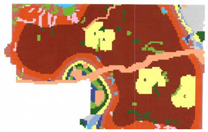
To apply this approach, experts can suggest the minimum area of high quality habitat necessary to maintain a given number of individuals of a target species. Given a map of habitat values, the ‘score’ of this minimum area can be determined. For example, a pair of kit foxes requires 1,036 ha. In their habitat map with cell size of 4 ha, they would need 256 cells of highly suitable habitat. Cells of highly suitable habitat is assigned a score of 6 points. Therefore, patches meeting the minimum size of 1,036 ha translates to a score of 1,536 habitat-value points.

Given a map of habitat values, the patches can be generated or ‘grown’ using a patch growing process. Simply, this spatial process begins by selecting a cell of highly suitable habitat and adding cells along its perimeter based on their suitability score.  The highest value cells are added until the patch meets the minimum habitat value score – 1,536 value points in the kit fox example.

Using this technique three core habitat patches (yellow) were generated for the kit fox, with some bordering or even incorporating lower value habitat (green).

Population defined core

Many species, including some top predators, do not defend discrete territories but range widely, overlapping with other individuals. For these, a commonly used metric is population density. In this case, core habitat is defined as an area that has a population density that exceeds a certain minimum density.

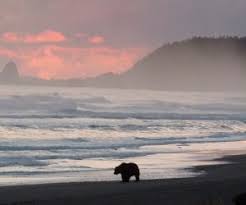
For example, we might consider core habitat for brown bears in Yellowstone National Park as an area that has a bear density of at least 1 bear per 50 square kilometers.

Territory separated core

In contrast to wide-ranging species, territorial species exclude other individuals from areas of habitat and thus space themselves more predictably across the landscape.

Their core habitat can be calculated based on how much habitat each territorial unit requires (R).

Circular areas of suitable habitat of size R can be super imposed on the landscape such that each area does not overlap. These areas are then considered core habitat.

In the example here, forty-seven territories were identified for spotted owls based on canopy closure and territory size requirements of the species.

The number of areas that can be superimposed on the landscape without overlapping is indicative of how many territorial units the landscape can support.

Population viability analysis

A method for modeling the effectiveness of a specific distribution of core habitat patches is population viability analysis. We will explore PVA more next week.
Identification of core areas is a necessary first step before connectivity across a landscape can be assessed, as covered in Topic 2.

Connectivity

Animals move across landscapes to acquire food, reproduce, migrate, and shift in response to environmental change. Most ecological processes happen within a spatial context that influences how those processes occur. The degree to which a landscape allows these flows to occur can be described as connectivity.

Defining Connectivity

Like many ecological concepts, there are several ways to define connectivity.

We’ll use this: the degree to which the landscape impedes or facilitates movement among resource patches (Taylor et al. 1993).

Measures of connectivity depend on the specific process of interest. For example, connectivity for foraging movements of a Chelan mountain snail are quite different from those of grizzly bears.

Why connectivity is important?

The persistence of many species across landscapes is influenced by their ability to move and recolonize areas when local subpopulations become extinct. Planning for habitat connectivity as a strategy can help plant and animal communities move in response to a changing climate.

Connectivity can also allow disturbances such as fire, insect outbreaks, and disease to spread. Awareness of habitat connectivity issues is growing among land management agencies and the public.

For examples, see:
• World Wildlife Fund’s Freedom to Roam
• Western Wildway Network

Ecological and theoretical background

There are two general ways to measure or consider habitat connectivity:

1. Structural Connectivity – The spatial arrangement of different types of habitat or other elements in the landscape.
   • Measures of structural connectivity quantify the characteristics and spatial arrangement of elements in a landscape (e.g. amount and distribution of a species’ habitat — sound familiar?)
2. Functional Connectivity – The expected behavioral response of individuals, species, or ecological processes to the physical structure of the landscape.
   • Measures of functional connectivity address the way an ecological process, such as the movement of individual animals, may be influenced by the arrangement of elements on the landscape

Modeling habitat connectivity

A model is a simplification of reality based on a series of assumptions about how a system works.

There are many types of ecological models:

• Conceptual models that synthesize existing information to allow a systematic exploration of the way we think a process works
• Statistical models that are based on quantitative empirical data
• Simulation models often combine conceptual ideas about how a system works with quantitative or empirical parameters to explore the process under different situations

Here we will focus on some of these approaches for modeling habitat connectivity, and we will explore additional facets of ecological modeling in the next lesson.

Considerations when modeling habitat connectivity include:

• Availability of core (source) habitat patches
• Boundary effects
• Connectivity among patches
• Quality of the surrounding environment (context)
• Dispersal ease or cost

Choosing analysis approaches

When choosing a connectivity assessment approach, consider the following questions:

1. What is the question to be addressed?
   Remember to clearly articulate the question. For example, a study question might be very specific and fine scale, such as “where along this 15-mi stretch of highway should crossing structures for painted turtles be located?,” or more broad, such as “which portions of California are least impacted by human activities and how are they connected?”
2. What is the simplest approach that will provide the needed information?
   Find the best trade-off between complexity and uncertainty. A good principle is to use the fewest GIS layers with the fewest classes that adequately address the question.
3. What is the scale of the question?
   Be careful to match the scale of analysis to the ecological processes under consideration.
4. Is the model testable?
   The best models allow us to determine if our understanding (e.g. of how animals move across a landscape) is correct. Strive to formulate the modeling question and output in a way that can be validated.

Tools and techniques

We will look at five approaches to connectivity analysis:

• Patch Metrics
• Graph Theory
• Cost-distance Analysis
• Circuit Theory
• Individual-based Models

All of these methods summarize spatial patterns that influence flows or movement across the landscape. In each, the intent is to distill highly complex patterns into simplified representations that can increase our understanding of how organisms or processes move across a landscape.

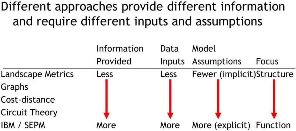
Connectivity analysis approaches range from the simple to the complex. In most cases, the choice of analysis approach involves a trade-off between the number of assumptions required and the amount of information provided by an analysis.

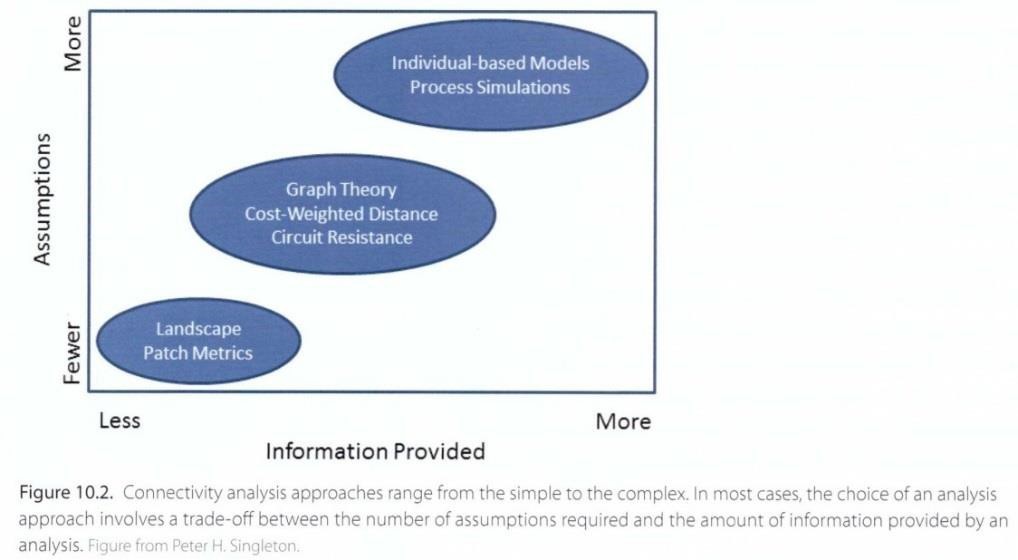
We will explore each of these approaches briefly, then delve deeper into cost-distance analysis and circuit theory.

Patch Metrics

Patch metrics summarize composition and configuration of elements in the landscape, and physically how connected they are (e.g. patch size, nearest neighbor, edge to area ratio). Patch metrics offer the simplest measures of structural connectivity across the landscape unit (e.g. watershed or planning unit). They are useful for quantifying and comparing landscape patterns at different times (e.g. historic range of variability or monitoring change) or different locations (e.g. comparing landscapes). However, patch metrics do not reveal functional connectivity – they don’t provide a lot of information about expected movement patterns.

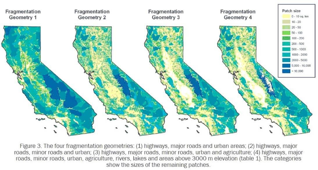
Patch Metric Example — Effective Mesh Size

Effective mesh size is a metric developed specifically to assess connectivity patterns. It quantifies landscape fragmentation based on the probability that two randomly chosen points in a region are located in the same non-fragmented patch. The more barriers (e.g., roads, railroads, urban areas) present in the landscape, the less chance that the two points will be connected. It can also be interpreted as the ability of two animals of the same species – placed randomly in a landscape – to find each other.

In the figure below, the state of California was fragmented according to different barriers to generate four ‘fragementation geometries’ (below).

Graph Theory

Graph theory is a collection of mathematical concepts that describes the relationships between things based on nodes (things being connected) and edges (the links between nodes). Graph theory is particularly useful for characterizing complex sets of patches and linkages forming networks. Most landscape permeability assessments are applications of graph theory that use different math methods for describing relationships between landscape features in a GIS raster layer.

Graph Theory Example

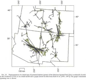
The habitat distribution for Mexican spotted owls is highly fragmented in the Southwest because suitable foraging and nesting sites are largely determined by topographic relief. Because of the arid climate and orographic effects, much of Mexican Spotted Owl habitat is divided into “sky islands” surrounded by grasslands and desert. Juvenile spotted owls are known to disperse considerable distances in search of vacant nesting territories. Thus it is highly likely that dispersal success plays an important role in the genetic, demographic, and metapopulation structure of the Mexican Spotted Owl.

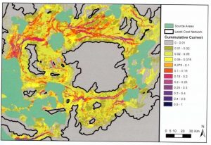
Graph theory was used to determine the likely routes of dispersal (edges, black lines) between suitable nesting sites (nodes, green) based on empirical data of owl dispersal and foraging behavior. This analysis shows if suitable habitat is effectively connected to other patches such that dispersal and occupation by the Mexican Spotted Owl is possible.

Cost-distance analysis

Cost-distance analysis is the most commonly applied spatial analysis technique for landscape connectivity analyses in conservation planning. ‘Cost’ refers to an energetic cost or risk of moving through the landscape from one ‘source’ or habitat patch to another.

Cost-distance analysis begins with creation of a resistance raster layer where each cell in the resistance layer is assigned an index of resistance or ‘cost,’ usually determined by the habitat characteristics at that cell. For each cell in the output cost-distance surface, the cost-distance algorithm calculates the product of the resistance index times the cell size for each cell in the least costly path to the closest habitat patch. The algorithm produces a continuous map of the cumulative resistance between each cell on the map and the most accessible habitat patch.

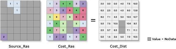
This algorithm produces two useful map products:

1. Least cost paths between two habitat patches, or the set of adjacent cells with the minimum cumulative resistance between two habitat patches.
2. Least cost corridors, or the set of cells for which the cumulative cost distance between two habitat patches falls below one or more user- defined thresholds.

NOTE: Cost-distance analysis can provide compelling representations of the relative permeability of different parts of a landscape but should not be interpreted as predicting specific movement routes through the landscape.

Cost-distance example

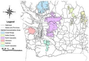
Here, we will explore the steps of cost-distance analysis for large carnivores – wolf, wolverine, lynx, and grizzly bear – in Washington State by Singleton and colleagues (2002).

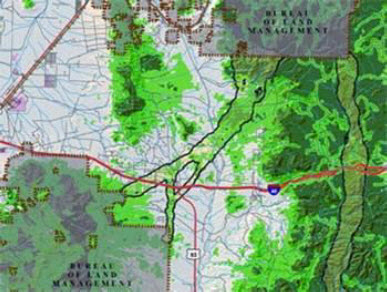
1. Identify source patches

   The map below shows large roadless areas and units highlighted in focal species management plans.

   

2. Develop friction surface

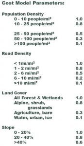Multiple data layers can be integrated to develop an index of resistance or ‘cost’ based on the habitat characteristics of each cell. The table below shows the resistance generated by different landscape characteristics.

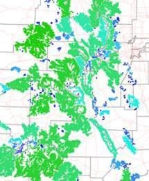
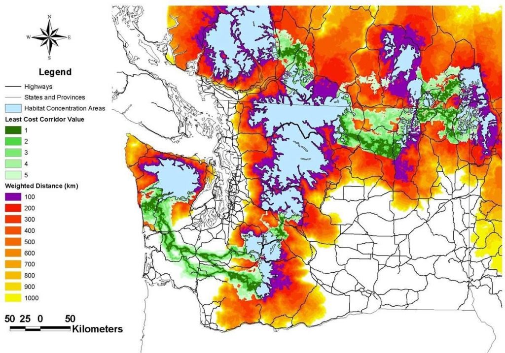
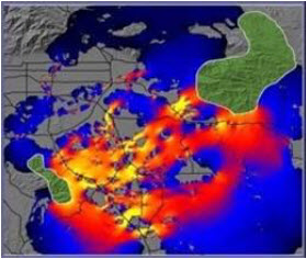
All of these resistance values can be combined through summation or weighting to generate a map of dispersal habitat. In the example below, habitat easy for animals to move through has a value of 1 and is shown in blue, while habitat that is difficult to transverse has a value of 0.01 and is shown in red.
This dispersal suitability can be transformed to generate a map of ‘weighted distances’ – a measure of the difficulty the species would have traversing a cell.

For example, a cell that is easy for animals to move through (dispersal value of 1) would have a weighted distance equal to its actual size – 90m. A cell that is difficult to traverse (dispersal value of 0.01) would have a distance of 9000m, meaning that crossing that cell would be just as difficult for the animal as traveling 9000m.

3. Calculate least cost distances

   Once the friction surface has been generated, the cost-distance algorithm calculates the product of the resistance index times the cell size for each cell to determine the least costly path between habitat patches.

4. Compare and plan

   With the least cost distance between habitat patches has been calculated, conservation planners can make informed decisions about how to improve connectivity by reducing the cost of moving between existing habitat patches, by creating new patches, or creating corridors.

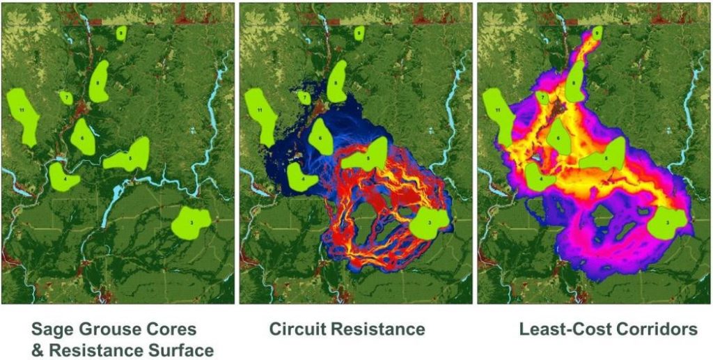
Circuit theory

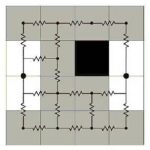
Based on electrical engineering theory, circuit theory uses networks of electrical nodes connected by resistors as models for networks of populations and habitat patches connected by movement.

This approach generates a measure of “flow” through each cell in a landscape. Using circuits as models for ecological networks is based upon a simple idea: multiple pathways in electrical networks increase connectivity. Thus, distance metrics based on electrical connectivity are applicable to processes that increase in magnitude with increased numbers of pathways.

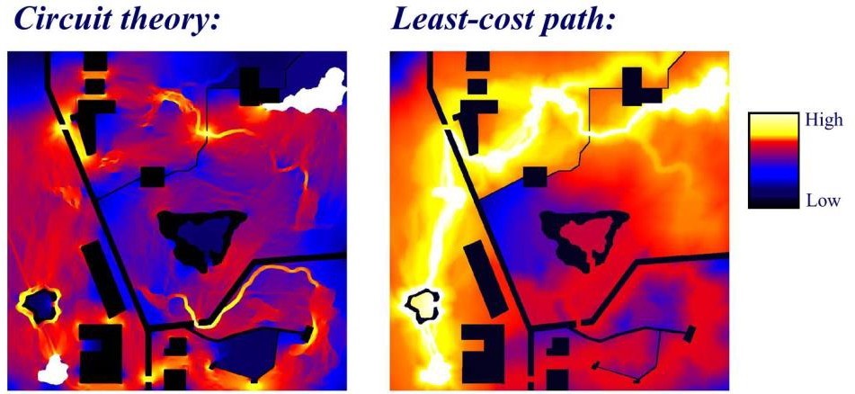
Let’s examine the connectivity between the two habitat patches circled below. Corridors mapped using cost-distance emphasize the “best” route through the landscape and assume that animals have perfect knowledge of the whole landscape.

More realistically, animals make routing choices based on their immediate surroundings and, in some cases, past experience and rarely have perfect knowledge of the entire landscape. In circuit models, all possible paths contribute at least somewhat to connectivity, and they reflect movement routes taken by ‘random walkers’.

Integrating cost-distance analysis and circuit theory

Circuit analyses complement least-cost path results by identifying important alternative pathways and ‘pinch points’ where loss of a small area could disproportionately compromise connectivity. Such areas can be prioritized for conservation action.

Circuitscape applies circuit theory to landscape connectivity analysis.

Individual based models and other approaches

Individual-based movement models (IBM) or agent-based models simulate movement of an individual through the landscape. They are built on the understanding that many ecological processes, such as metapopulation dynamics and range shifts, emerge from the behavior of individuals, and the behavior of each of those individuals can be simulated in a manner than allows modelers to investigate the emergent processes of interest. These models are mechanistic, incorporate stochasticity, and are more focused on assessing functional connectivity. They can be applied at many scales, from dispersal (coarse) to foraging (fine).

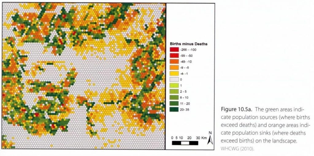
Population viability models (PVA) use demographic information to project population persistence and complement individual-based movement models by identifying population sources and sinks (Fig 10.5a).

Spatially explicit population models (SEPMs) integrates PVA with a heterogeneous landscape to simulate interactions of landscape features, species movement, and demographics.

We will look at some of these tools more in the next lessons.

Choosing an approach

All of these modeling approaches involve major assumptions about:

• Habitat associations
• Parameterizing source areas or habitat patch characteristics
• Dispersal behavior
• Resistance to movement

Topic 2 Knowledge Check

Applying core and connectivity tools in GIS

Application of cost-distance analysis:

This study presents an example of performing a cost-distance analysis for Redstart (phoenicurous phoenicurous), an umbrella species for woodland birds, conducted by Nikolakaki (2004). We suggest taking the time to read this paper (provided as a pdf), as it illustrates cost-distance analysis very effectively.
This example uses a GIS approach to first identify suitable habitat (source patches) and then estimate the connectivity of habitat patches based on the redstart’s landscape requirements. Each patch is assigned a “cost” value that represents the cost of dispersal over a friction surface. The sites are ranked accordingly and, in combination with the spatial context and size, are prioritized in terms of their potential for forming cores for habitat creation.

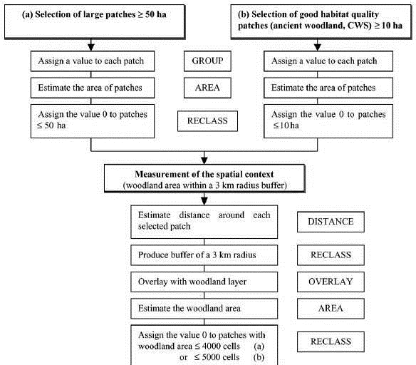
Redstart landscape requirements:

• 0.6-0.8 pairs/ha territory size
• A minimum size of 5 ha was assumed to support a local population of 3-5 breeding pairs.
• Habitat patches of 50 ha or more of mature deciduous woodland could support a population of 30-50
• Woodland within a 3 km radius = predictor of the degree of isolation.
• During the breeding period, daily movements across arable land range from only a few hundred meters up to approximately 700 m.

Methods for identifying priority sites for conservation

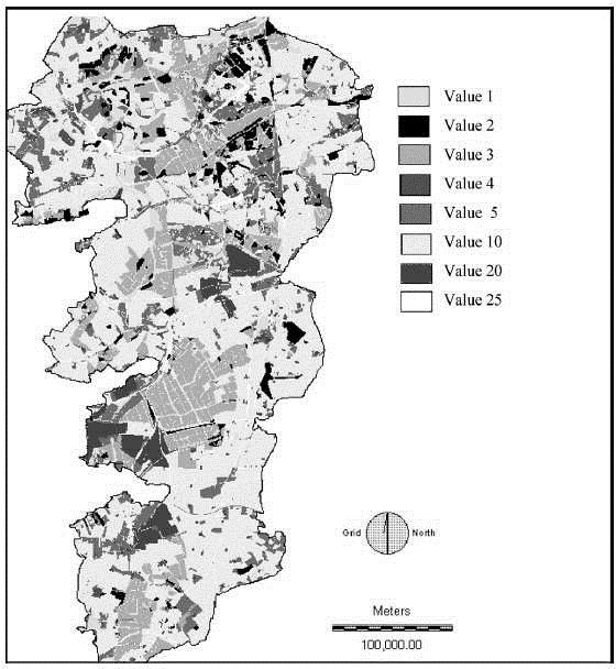
Step 1: Identify source patches. Areas of suitable Redstart habitat are identified based on the habitat requirements of the species, as illustrated in the diagram below.

Step 2: Create a friction surface for Redstart movement based on the species’ landscape requirements. Here, a ‘cost’ value is assigned to each cell based on land cover characteristics. Areas through which the Restsart can move most easily were assigned the lowest value (1), and areas highly resistant to movement were assigned the highest value (25).

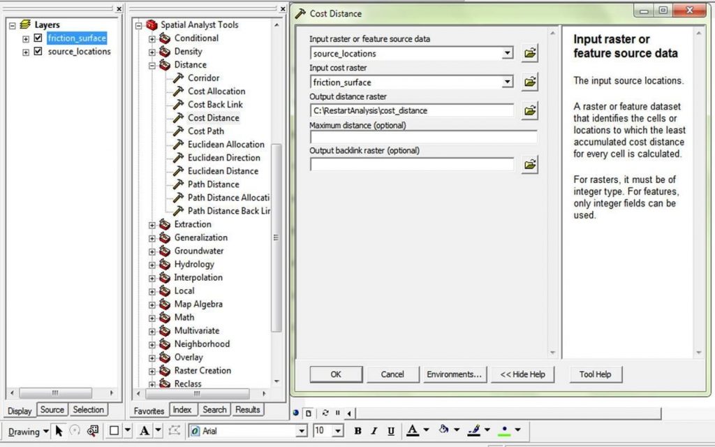
Step 3: Create a cost-distance surface. Using the Cost Distance tool, part of the Spatial Analyst toolbox, the raster layer identifying source patches (from Step 1) and the friction surface generated (from Step 2) are used to create a cost-distance surface for the species.

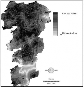The resulting cost-distance surface shows areas through which the Redstart can freely move in black, and barriers to movement in white. Conservation efforts can use this map to highlight locations in which to target restoration activities to improve connectivity for the Redstart.

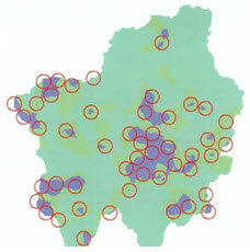
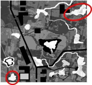
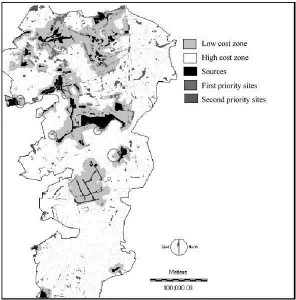This analysis enabled identification of priority sites for habitat creation (below). Sources are shown in black; the grey area around the sources indicates the low cost zone, and the white area the high cost zone. The darker grey patches within the low cost zone are the first priority sites for habitat creation; those in circles represent the high priority sites. The patches within the high cost zone are the second priority sites.

Exploring tools for connectivity analysis

More tools are available! Click the links to explore the tools below designed to facilitate connectivity analysis in the ArcGIS framework.

Circuitscape is a free, open-source program that can be called up as an ArcGIS toolbox. Circuitscape borrows algorithms from electronic circuit theory to predict connectivity in heterogeneous landscapes.

Corridor Designer includes an ArcToolbox for creating habitat and corridor models with ArcGIS and an ArcMap extension for evaluating corridors.

Topic 3 Knowledge Check

References:

Brodie JF, Giordano AJ, Dickson B et al (2015) Evaluating multispecies landscape connectivity in a threatened tropical mammal community. Conservation Biology 29(1):122-132

Freeman RC, Bell KP (2011) Conservation versus cluster subdivisions and implications for habitat connectivity. Landscape and Urban Planning 101(1):30-42

Nikolakaki 2004