2 Lesson 2: Viability and Optimization Lesson

Viability and Optimization Lesson

In this lesson you will:

• Distinguish among concepts and methods for measuring viability of a population or species in a current or planned landscape
• Learn practices and applications of population viability models
• Understand optimization concepts and models in the context of reserve design problems
• Identify optimization methods, algorithms, and decision support systems used to select reserve sites
• Evaluate how simple optimization models can be used for reserve site selection and design

Chapters 11 and 12 in Craighead and Convis accompany this lesson.

Lesson Topics

This lesson will cover three topics and take approximately 40-50 minutes to complete. We recommend working through each topic in the order in which they are listed below. You may return to this page at any time by clicking the ‘Home’ button at the bottom of the page.

1. Spatial planning to ensure viability of populations
2. Reserve design and optimization
3. Applying reserve design

Spatial planning to ensure viability of populations

Introduction

Suppose you now have a good understanding of the study landscape, what focal species you might use to represent ecosystems of conservation concern in your area (such as the California spotted owl), and the habitat available to those species.

You have even mapped out areas of suitable habitat and analyzed the connectivity between potential conservation areas.

However, merely protecting areas of suitable habitat does not necessarily ensure that the amount and configuration of habitat patches will be sufficient for the long-term survival of the focal species.

Likewise, even if sufficient amounts of suitable habitat are available, species may still decline due to threats unrelated to habitat loss, such as harvesting, introduced predators, competitors, or diseases.

Population Viability Analysis

Assessing viability is the most direct way of measuring how close your conservation plan is to achieving protection of target species.

Viability is the likelihood that a species (or a population) will remain extant. Questions of viability occur mostly at the population level, which for many focal species requires regional-scale analysis.

Population viability analysis (PVA) is a method for calculating this likelihood, either under current conditions or under assumed future changes.

Population viability analysis (PVA) provides a method to link demographic data with habitat maps to address questions about the prospects for recovery, longevity, and resilience specific to focal species in your landscape.

PVA can be particularly useful when evaluating different management options or proposed reserve design configurations, and for prioritizing research and data collection needs through the use of sensitivity analysis. For example, habitat loss may result in smaller populations, which may make them more vulnerable to effects of hunting.

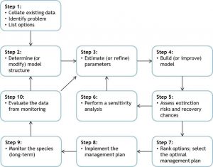
Practices and components of PVA

PVA is a process of predicting measures of population persistence, such as risk of population extinction or decline, chance of population recovery, expected future population size, and expected time to extinction. Therefore, example PVA results may include:

• Probability of extinction within the next 100 years
• Probability of a 50% decline by the year 2060
• Probability that there will be 50 or fewer mature individuals left
• Probability that the population will increase to 1000 or more individuals by 2050

PVA uses a variety of models – parameterized with habitat data, distribution data (e.g. occurrence locations), and demographic data (e.g. censuses, dispersal events) – and relies on information about the ecology of the species (e.g. life stages). Though there is no single recipe to follow when performing PVA, the main components are outlined below.

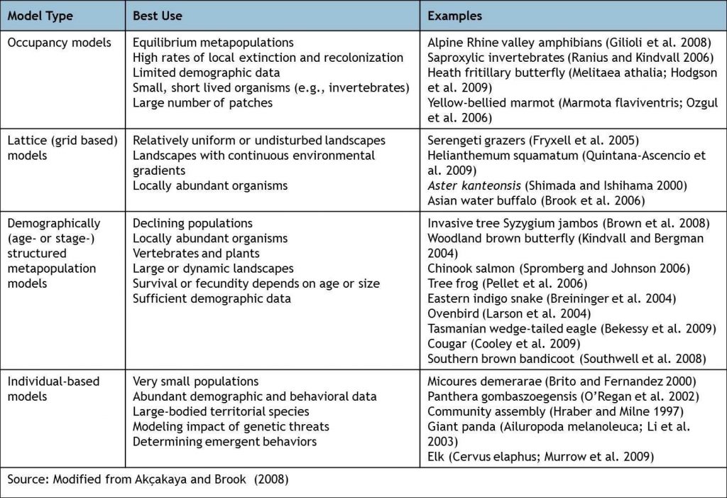
Types of PVA Models

There are several types of PVA models and several software packages available to implement them.

Questions addressed with PVA may involve:

• Assessing vulnerability
• Impact assessment
• Evaluating management options
• Planning research
• Improving understanding

Assessing vulnerability

Estimating the risk of extinction (an absolute measure of vulnerability), or the relative vulnerability of species and populations to extinction.
These predictions can be used in ranking species (such as in the IUCN Red List of Threatened Species). When combined with such considerations as cost-effectiveness, social and cultural priorities, and taxonomic uniqueness, these results can also be used to set policies and priorities for allocating scarce conservation resources.

For example, the IUCN has used PVA to give the red panda a ranking of vulnerable, because its population is estimated at less than 10,000 mature individuals with a continuing decline of greater than 10% over the next 3 generations.

Impact assessment

PVA can be used to quantify the impact of human activities (such as urban sprawl and other types of land-use change; harvest, poaching, and other types of direct exploitation; pollution; and introduction of exotic species) by comparing results of models with and without the population-level consequences of the human activity. These assessments may involve past or current impacts (to assign responsibility) or projected future impacts (e.g., to evaluate proposed development plans).

For example, PVA has been used to estimate the impact of poaching on elephant populations.

Evaluating management options

Predicting the likely responses of species to conservation can guide management actions, such as reintroduction, captive breeding, prescribed burning, weed control, habitat rehabilitation, or different designs for nature reserves or corridor networks.

For example, PVA could be used to plan for reintroduction of captive- bred species into the wild, such as the black footed ferret. This species was considered extinct in the wild in 1987 but has been reintroduced into eight western states and Mexico from 1991–2008. There are now over 1,000 mature, wild-born individuals in the wild across 18 populations.

Planning research

PVA might also be used in determining priorities for further data collection. Research priorities might be based on the sensitivity of PVA model results to data uncertainties in model parameters.

Improving understanding

Finally, PVA might help in organizing the information and assumptions about a species or a population. PVA allows a structured process that makes the assumptions explicit and highlights the data deficiencies and uncertainties.

Preliminary Data Considerations

Before you begin PVA, it is important to clearly identify the question you wish to answer with your analysis (you’ve heard that before!). The goals and the specific questions of a PVA, and the particular scenarios to be explored, should be developed in the course of a participatory process in which both experts and stakeholders outside of the professional scientific community provide input.

A habitat map is the spatial backbone of a PVA and directly relates to many demographic parameters, such as the number and carrying capacity of subpopulations and dispersal rates. Therefore, most PVA’s with spatial structure start from a map of suitable habitat for the modeled species.

Another important consideration when constructing a model for a PVA is the spatial scale of your data, both in terms of the resolution and the extent. The scale should be relevant to the biology of the focal species, meaning it should relate to the patch size and dispersal distance.

A good guideline for vertebrate species is that the cell size of the raster map underlying the model should be smaller than the home range or territory size of the species.

PVA Modeling Components

Here, we outline some of the key PVA model components one should consider before applying PVA. We will focus more attention on these six issues:

• Demographic structure
• Density dependence
• Spatial structure
• Dispersal & connectivity
• Variability & uncertainty
• Landscape change

Demographic structure

Demographic structure refers to the categorizations of individuals within a population according to their age, size, sex, or physiological stage.
Models should have an age or stage structure if the demographic characteristics depend on the age, size or other characteristics of the individual. These matrix models (named so because of the way demographic rates can be organized in a matrix equation) are commonly used in conservation biology and can be parameterized using mark and recapture data and population censuses. Many demographic models include only females.

Models that lack age or stage-based structure are called scalar models – which assume all individuals in the population are functionally identical. Scalar models are used when the only available data is a time series of total population estimates.

Density dependence

Density dependence refers to how the population growth depends on population size. Typically, survival and fecundity decrease as a function of population size due to intraspecific competition for limited resources (food, light, space).

Density dependence can have important effects on extinction risks. Therefore, it is necessary to use caution when selecting the type of density dependence and specifying its parameters.

• Most types of density dependence are modeled with two main parameters:
  Max population growth rate (Rmax)
•  Carrying capacity (K) – the population size that can be supported by available habitat and resources – an important link to habitat map

Spatial Structure:

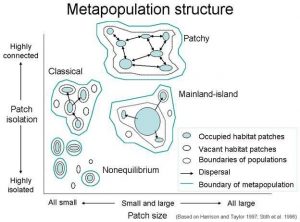
Most PVA models represent the landscape as discrete patches of suitable habitat surrounded by a matrix that may support dispersal. Each discrete habitat patch is assumed to support one biological population. How these populations are configured (i.e., the number, size, shape, and location of these populations on the landscape) determines the model’s spatial structure.

One approach to delineating populations is to identify clusters of ‘highly suitable’ cells in a habitat suitability map based on a distance parameter, or ‘neighborhood distance.’ Individuals that are farther apart than the neighborhood are considered in different populations.

Dispersal is the movement of individual in the landscape. Dispersal between populations allows sinks to become recolonized and decreases the probability of local extinction (rescue effect).

How connectivity is incorporated into PVA depends on model type. As you saw in Lesson 1, parameters to model connectivity commonly include:

• dispersal rate – proportion of individuals moving from one habitat patch to another per unit time. This can be estimated from the least-cost path (or friction) maps that we learned about in the last Lesson.
• dispersal probability – probability of an individual moving from one patch or cell to another within a given time interval

Some variability in population sizes arises from the internal dynamics of the population (e.g. fluctuations in age composition).

Demographic stochasticity is the sampling variation in the number of survivors and the number of offspring that occurs, because a population is made up of a finite number of individuals. Relative to other factors, demographic stochasticity becomes more important in small population sizes.

Variability is also caused by fluctuations in environmental factors, causing stochastic changes in demographic rates such as survival, growth, fecundity, and dispersal.

Estimating temporal variability of demographic rates for a PVA is often complicated. For a summary of methods for estimating demographic variability, see pages 282-283 in Craighead and Convis.

Landscape change causes changes in the spatial structure and characteristics of populations, which can have important effects on the viability of the species.

For many species, habitat loss and global change are two threats that cause reduction, shifts, and fragmentation of their habitats. To adequately address these threats, a PVA should allow dynamic spatial structure – it should simulate temporal changes in the location and number of populations that arise from habitat patches splitting, merging, appearing, and disappearing as the species’ habitat changes.

Tips for Model Application

Remember, all models rely on assumptions. It is important to be mindful of the explicit assumptions you are making in your model as well as the assumptions that are implied through the model parameters, and always evaluate whether they seem reasonable or supportable within the context of the question you are trying to address. Model assumptions often play a key role in determining the ‘fit‘ of a model, or how well it simulates the phenomena of interest.

A good way to test the fit of a model is to use separate, independent data for model building and model validation. Separating training data and testing data can come from partitioning a single dataset spatially or temporally. For example, a model of habitat suitability might be constructed using known occurrences in half of the landscape then tested for accuracy by seeing how well it can predict the occurrences in the other half.

Sensitivity analysis enables assessment of the relative effects of uncertainty in model parameters on model results. This information can:

• help identify important parameters in which small changes in estimated values or assumptions have relatively large effects on conclusions drawn from the model
• help to prioritize resource allocation for collecting field data to inform further modeling efforts.

Guidelines for implementing conservation using PVA

Evaluating conservation options

When making decisions between multiple management options, very often the final decision depends on a combination of both biological (i.e., the long term viability of the focal species) and non-biological considerations (i.e., the societal, cultural, of financial constraints associated with the proposed action). PVA can be used to evaluate and rank different conservation options by providing a biologically-based risk assessment. Decision makers can then decide if it is more important to maximize viability for the species or minimize the costs.

Critical habitat

Often the designation and protection of habitat critical to a threatened species’ survival is proposed or required. PVA models can be used to compare different scenarios for the amount and configuration of habitat to place under protection to determine the resulting viability of the species under each scenario.

Climate and environmental change

PVA models can be used to couple species demography and changes in the landscape, allowing modelers to examine how a species’ dispersal and colonization abilities will be able to keep pace with the rate of change. Some work on this demonstrates how a species’ risk of extinction under climate change depends on complex interactions between life history characteristics and the landscape (Keith et al. 2008, others). Linking PVA to climate models starts with interpolating the climate predictions to create a time series of available habitat maps.

Cumulative impacts

An important advantage of PVA compared to other methods of assessment is that it can simultaneously incorporate the effects of multiple impacts (i.e., habitat loss, climate change or harvesting) and conservation measures (i.e., habitat corridors, restoration, or reintroduction).

Reserve selection and design models

Conservation scientists have long grappled with how to best design nature reserves.

Size and configuration determine how well certain species and ecosystems are protected. Reserves must also support landscape dynamics and address external impacts.

Optimization, drawn from military and business logistics, provides a systematic process for reserve selection and design.

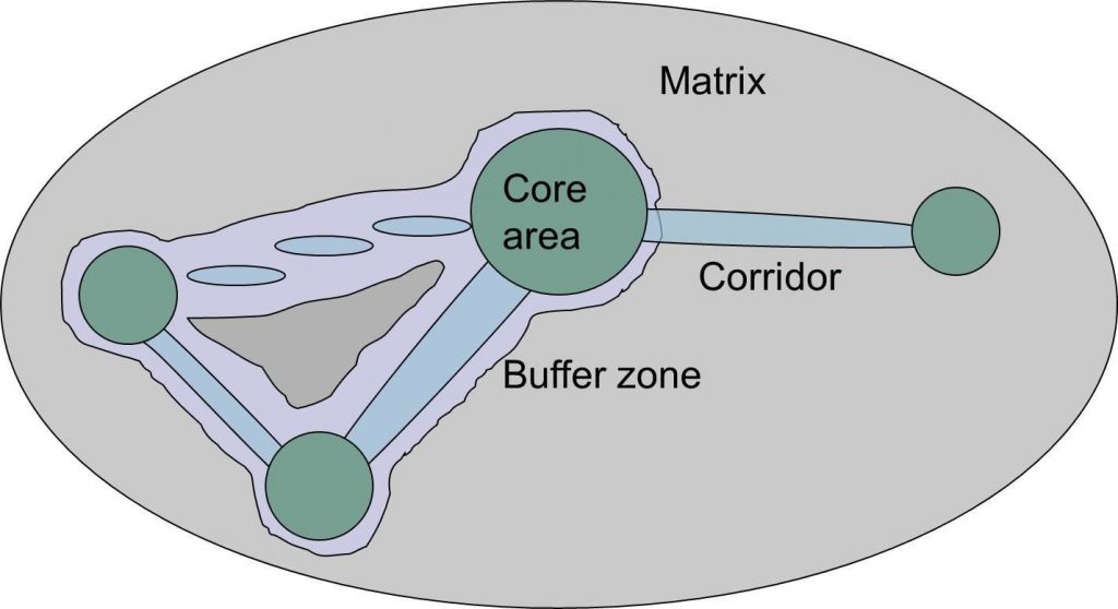
Geometric elements of reserve design

We will use specific vocabulary when discussing the elements of reserve design. Some of these concepts should already be familiar from previous lessons.

1. matrix – the intervening area in which a set of habitat patches are situated. The matrix may be more or less hospitable to species movement.
2. core – an area or patch of relatively intact suitable habitat that is sufficiently large to support more than one individual of a species.
3. corridor – a strip or ‘stepping stones’ of land linking two or more protected areas to promote connectivity and allow movement of individuals between otherwise isolated patches of core habitat. Corridors may be patches of suitable habitat too small to support species long term or areas with low resistance to movement.
4. buffer zone – an area of low intensity disturbance or human use surrounding a strictly protected core or corridor area.

SLOSS: Principles of Reserve Design

Diamond (1975) and others proposed geometric reserve design principles based on island biogeography that have come to be known as the SLOSS guidelines (single-large-over-several-small). The authors observed how species dispersed and persisted in an island archipelago. These guidelines suggest better versus worse reserve configurations:

1. A large reserve is better than a small reserve.
2. The reserve should generally be divided into as few separate pieces as possible
3. If the available area must be broken into several reserves, then these reserves should be as close to each other as possible.
4. If there are several separate reserves, these should ideally be grouped equidistant from each other rather than grouped linearly. This configuration ensures that the loss of one would not reduce connectivity between remaining reserves.
5. If there are several separate reserves, connecting them by strips of the protected habitat (corridors) may significantly improve their conservation function.
6. Any given reserve should be as nearly circular in shape as other considerations permit (smallest edge-to-area ratio) to minimize edge effects and dispersal distances within the reserve.

In the following pages, we will practice applying these guidelines.

Reserve design and optimization

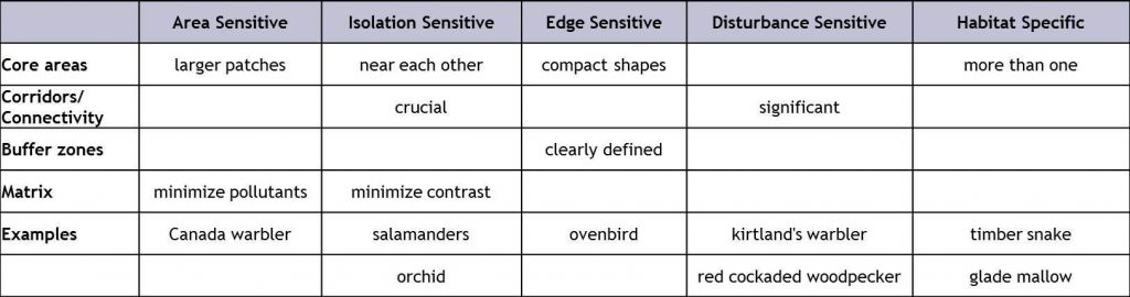
Modeling for species sensitivities

The table below illustrates how reserve geometry can be used to accommodate specific sensitivities of target species.

Optimization Models

While SLOSS provides a useful starting point, reserve design depends more on what one is trying to protect within the context of available options. Because conservation resources are typically very limited, conservation design often seeks to answer questions like ‘what is the minimum number of reserve sites necessary to represent all species of concern?’ or ‘what is the maximum number of species that can be represented for a fixed budget?’

In response, conservation practitioners developed systematic and strategic reserve site selection approaches that evolved into the optimization and decision support systems we use today.

Optimization models are ‘prescriptive’ in that they seek to identify a good or best course of action from among many possibilities. The optimal solution will at least point toward what is best, or can assess what is needed.

Some researchers distinguish between reserve site selection and reserve design models. Site selection models do not account for spatial attributes, such as connectivity and compactness, in the selection process. Reserve design models employ spatial metrics, such as inter-site distance and site adjacencies, and the resulting solutions are likely to be more spatially coherent.

Decision Support Systems

The need to generate, evaluate, and display alternative reserve plans rapidly has led to the development of computer based decision support systems (DSS) – interactive software systems that will help the user compile raw data documents, personal knowledge, and models to identify and solve problems and make decisions.

In the first step – formatting, reading, and analyzing input data – a DSS may interface with GIS. GIS data utilized by a DDS may include species presence data, land cover or land use layers, and socioeconomic data. The GIS may also generate new data based on map overlays of other datasets.

The second step – processing – is where optimization models come into play.

In the third step, the DSS may create full color map outputs (using GIS) that show the sites that have been selected for the reserve system.

Example DSS for reserve site selection

• 

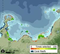
  Marxan – designed to select sites so as to minimize the total area (or cost) of the reserve system. The Nature Conservancy used Marxan in a prioritization of marine conservation zones in Kimbe Bay, Papua New Guinea (right). We will learn more
  about Marxan in Topic 3.

• Zonation – begins with the full landscape
  and iteratively removes sites one at a time until only the desired reserve system remains

Applying Reserve Design

In this topic, we will see how reserve design is applied through exploration of the following case study:

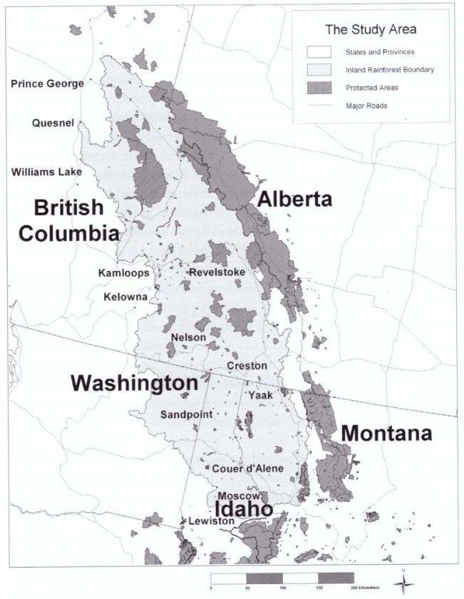
Site selection models for the North American Inland Rainforest –

An optimization model used with ArcGIS.

Background

Using approaches described in this lesson, the team developed a habitat suitability model for identifying high-quality and critical habitat for each of 6 focal species – cougar, grizzly bear, lynx, wolf, wolverine, and mountain caribou. The identification of core habitat provided the basis for selecting tracts of land in both Canada and the U.S. that would be recommended for protection in the Inland Temperate Rainforest Conservation Area Design. It was not practical to protect all of the core habitats, so a target area of core habitat was defined for each species. The goal was to satisfy all targets simultaneously in the most efficient way – with a minimum total number of sites.

Data

The Inland Temperate Rainforest was partitioned into 1km grid cells. Those cells that met high quality thresholds for at least one of the six target species were designated as core habitat. This classification was analogous to species presence/absence data in that a yes or no designation was made for every focal species.

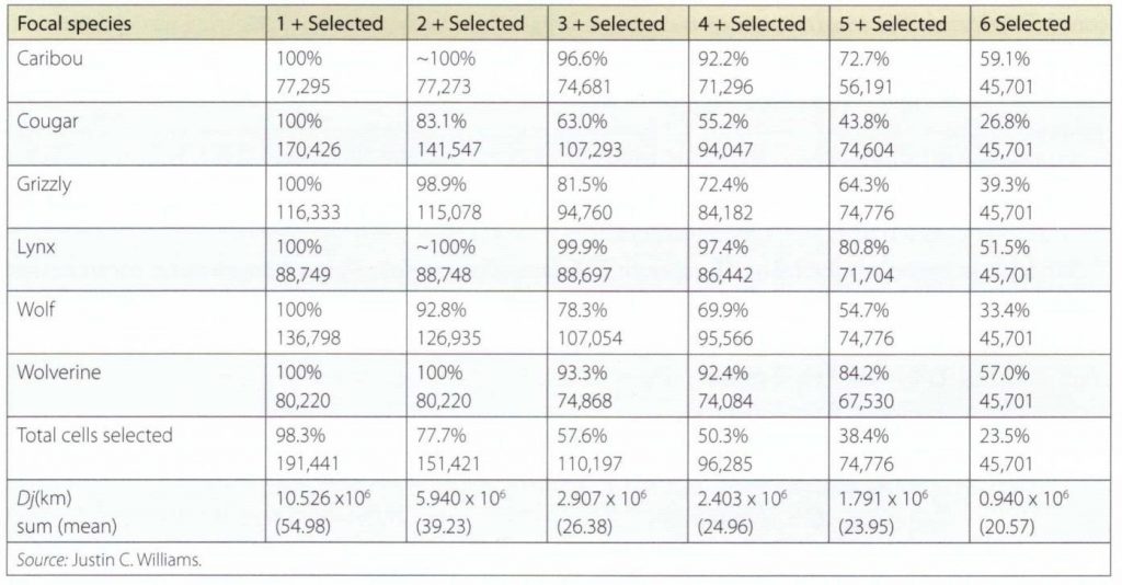
Methods and Results

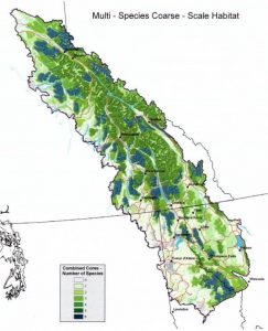
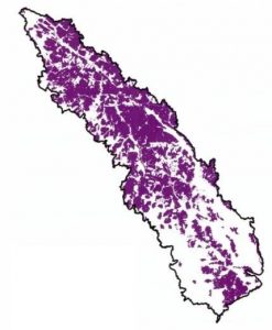
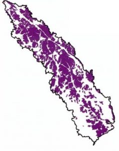
The composite core method is a simple but effective rule for generating reserve designs and resulted in six alternative designs for the Inland Temperate Rainforest. The first alternative, which is the largest in terms of total area, was generated by selecting all cells that were core for any ONE of the six focal species. The second alternative was generated by selecting all cells that were core for any TWO of the six focal species, and so on. The map to the right shows the composite cores nested in terms of the number of focal species whose habitat is represented. The table below shows the amount of core habitat selected for each focal species in each alternative.

Optimization Models

Three optimization models were also defined:

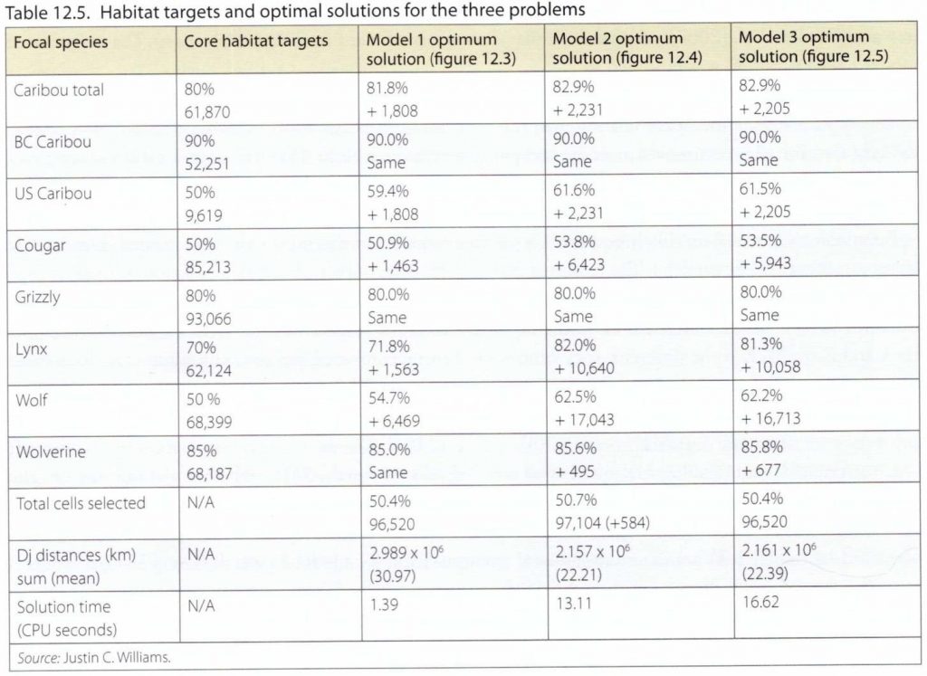
Model 1 was designed to identify a reserve with the smallest total area, which can then be used as a baseline of comparison for the composite core solutions and for the optimal solutions of the other models. A variation of the minimum reserve set model, this model had a goal of minimizing the total amount of core cells selected while meeting or exceeding a specified number of core cells for each species (50% of habitat cells). This model resulted in the smallest total reserve area (96,520 km squared) as shown in the map to the right, but did not promote compactness or connectivity. The mean distance of habitat cells to the nearest neighboring patch was 30.97 km.

Model 2 was designed to promote compact clustering of selected habitat around naturally occurring habitat clusters. This model utilized the cluster analysis tool in ArcGIS to identify discrete clusters of core habitat for each species. For each core habitat cell, the closest cluster was identified and a distance coefficient was determined for each cell. The model then selected cores to minimize the total number of distance-weighted cells selected. The resulting design shown in the map to the left contained a slightly larger area (97,104 km squared) but more compact, less fragmented reserve design than in Model 1.The mean distance of habitat cells to the nearest neighboring patch was 22.21 km, 28% lower than Model 1.

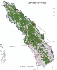Model 3 minimized distance as in Model 2, except that the total area was limited to the area selected in Model 1 (96,520 km squared). Therefore, model 3 encouraged clustering of selected cells and meets the core habitat targets for each species but uses no more than the minimum total area necessary. The mean distance of habitat cells to the nearest neighboring patch was 22.39 km.

These models can be used to identify the trade-offs between total area, coverage in excess of targets, and reserve compactness. Much of the value of optimization is found in generating these tradeoffs.

Optimization Model Results

The table below shows the area of core habitat protected for each target species by each optimization model.

The role of optimization models in conservation planning

Optimization models are tools for decision support as opposed to decision making. Their purpose is to provide guidance, information, and insight for planning and decision making – not to dictate a course of action.

Optimization models provide several benefits for reserve design:

• model formulation produces a concise, exact statement of the problem
• they are highly general and can be transferred from one setting to another, one dataset to another, or (potentially) one spatial scale to another
• the optimal solution can establish benchmarks or baselines for the criteria being modeled that can help put other (perhaps more practicable) alternatives in perspective
• they can be used to generate alternative designs
• they can be formulated to address a wide array of issues that may influence reserve design

Marxan is a decision support tool for reserve design and is the most widely adopted site selection tool by conservation groups globally. Marxan seeks to identify efficient areas that combine to satisfy a number of ecological, social and economic objectives.

Given data on species, habitats, ecosystems and other biodiversity features, Marxan was designed to minimize the cost of selected sites while meeting all representative goals. Watch the video below to learn more about the reserve design principles underlying Marxan.

How to choose marine reserves

Marxan Methods

Here, inputs, process, and outputs generated by Marxan are briefly summarized. Visit The Nature Conservancy’s Marine Planning website to review several real-world examples of multi-objective planning efforts to address energy development, fisheries, coastal hazards, biodiversity conservation, and marine zoning that have been aided by Marxan.

In Lab this week, we will gain hands on experience applying Marxan to aid in conservation planning.

Process

The overall objective of the Marxan process is to minimize the area encompassed with the network of selected sites. To this end, Marxan evaluates alternative site selection scenarios, comparing a very large number of alternatives to identify a good solution. A scenario in Marxan is a user-defined set of parameters including the desired number of solutions or runs and the amount of aggregation or clumping of assessment units.

The procedure begins with a random set of units, and then at each iteration, swaps assessment units in and out of that set and measures the change in ‘cost.’ Cost here means the amount of area selected in the alternative. The algorithm’s function is a nonlinear combination of the total area and the boundary length of perimeter of the site selection output.

Inputs

1. The suitability index is a compilation of factors that generally includes impacts, threats and human uses that significantly influence where sites will be selected.
2. The boundary length modifier determines the level of assessment unit clumping or adjacency.
3. The species penalty factor determines the priority in which each individual target or feature can accomplish its goal.

Outputs

The two most widely used solutions provided by Marxan are:

1. Sum solution – reports out on all of the runs or solutions from a given scenario. This keeps track of how often each unit was involved in any solution. So if the user chooses the program to run one hundred times in a particular scenario, then the output reports on how many times any specific assessment unit is selected out of a hundred. This information is a useful way to explore the replace- ability of units. A “sum of sum solution,” or multiple scenarios added together, has also been referred to as an irreplaceability analysis.
2. Best solution – the most optimal run in the scenario that best meets the defined parameters. The objective function states that the best or most efficient solution will be the selected sites at the lowest total cost. While useful, planning teams have generally chosen to run Marxan by varying parameters and comparing best solutions. This increases the flexible nature of the site selection process and can trace patterns of representation across scenarios. This is extremely helpful for highlighting areas that have previously been overlooked, where goals for many targets can be met in a spatially cohesive manner that increases the likelihood of strategy effectiveness.

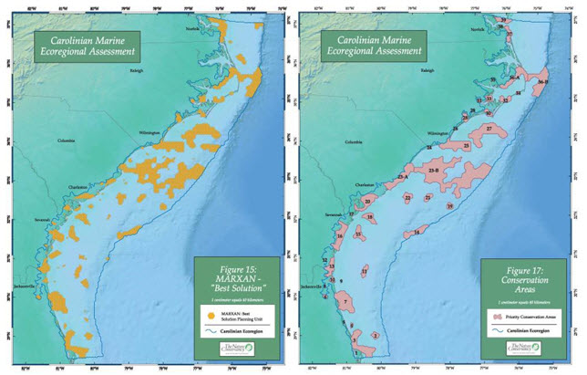
Example

In the Carolinian ecoregion, Marxan was used to identify efficient solutions that met conservation goals for all targets (left map); these
results were evaluated and modified in expert workshops (right map).