
3 Lesson 3: Landscape Modeling
Landscape Modeling
In this lesson you will:
- Learn the basic principles underlying spatial modeling
- Learn key considerations for landscape model selection and application
- Consider different approaches and uses of landscape scenarios
- Explore an application of forest landscape scenario modeling in the Upper Peninsula
Parts of this lesson are drawn from Chapter 14 in Craighead and Convis, Mapping biological processes to the appropriate spatial modeling tools. Other examples in this lesson are drawn from our own research.
Lesson Topics
This lesson will cover three topics and take approximately 50-60 minutes to complete. We recommend working through each topic in the order in which they are listed below.
Introduction to Models
Introduction
The goal of a conservation plan is to maintain or enhance biodiversity, ecosystem function, and ecosystem structure while accommodating human-oriented land uses. We can design and evaluate models that integrate the biological processes we are trying to maintain with socio- economic considerations.

Here, we define a biological process as a series of events generally occurring over time between living species interacting with one another and with the landscape. Examples of biological processes include:
- Snow leopards moving through a landscape
- Trees reacting to a fire burning through an area
- Wolverines adapting to changes caused by a warming climate
What are models?
As you’ve heard before, a model is an abstract representation of a system or process. Models can be physical, verbal, graphic, or mathematical.
Most of the models used in landscape conservation and planning are mathematically-based and spatial. These models are derived and implemented with the help of computational software – from statistical packages to GIS.
Mathematical models describe a process or system using mathematical concepts and language (known or estimated numerical relationships, coefficients and formulas). In a statistical regression model for example, one or more variables can be changed in the model to produce different results.
A spatial model is needed when the variables or processes of interest have explicit spatial locations. In addition to representing the process or system mathematically, spatial models also characterize the spatial relationships, such as spread of disturbance.
Why do we need models in conservation?
- They help us define problems more precisely and concepts more clearly.
- They are useful in situations where experiments are impractical or impossible.
- They provide a means of analyzing data and communicating results.
- They, perhaps most importantly, allow us to project into the future.
Under the Hood
Underlying all models are:
- Mathematical or spatial algorithms
- Assumptions
- Empirical data
- Expert knowledge
Models are usually a continuum of parts, processes, and empirical
estimations. Modelers MUST be aware of and understand all of these to apply a model and interpret results properly.
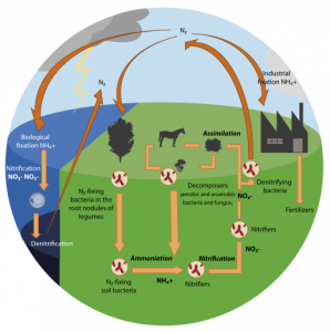
For example, a model of the nitrogen cycle might begin as a conceptual model describing what we know about how this system works. Empirical data might be used to develop a mathematical model or series of equations describing the relationships between the different processes in the cycle and the rates at which they occur.
Understanding what aspects of the biological process a model captures and what aspects it does not, provides insight into interpreting model results.
From the nitrogen cycling example, the contribution of earthworms to the breakdown of organic matter and its effect on the nitrogen cycle may not be well-characterized in the literature. Options might include the use of expert knowledge to complete the model or, in some cases, assumptions must be made to compensate for a gap in knowledge.
Vocabulary
We tend to use a specific vocabulary to describe the components of models:
-
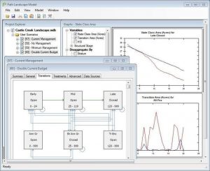
Screen shots from Path landscape modeling program Parameter – constant or coefficient that does not change in the model
- Variable – quantity that assumes different values in the model
- State variable – describes the mathematical “state” of a dynamic system. For example, a state variable in a model might be tree age. Age can change to a
new ‘state’ through model runs. - Rate variable – determines the rate of change of a state variable is given by a differential equation. Here the model would define the growth rate of a tree as it ages. We would expect this rate variable to be different for different trees, and the rate of growth could change under, say, changing climate.
- Output variables – variables that are computed within the model and produced as results. Reliable estimates for both state and rate variables allows us to more accurately project the value of the output sate variable (e.g. tree age, size) in the future.
- Initial conditions – values of the state variables at the beginning of a simulation
- Forcing function – function or variable of an external nature that influences the state of the system, but is not influenced by the system (e.g. changing climate on growth rates)
Further specific terms are used when discussing the modeling processes:
- Calibration – process of changing model parameters to obtain an improved fit of the model output to empirical data
- Sensitivity analysis – methods for examining the sensitivity of model behavior to variation in parameters – you have already used this!
- Validation – commonly the process of evaluating model behavior by comparing it with empirical data, some prefer the term corroboration because it does not imply ‘truth’
- Verification – process of adjusting the model code for consistency and accuracy in its representation of model equations or relationships
Basic Steps in Building a Model
To model biological processes, the spatial relationships of the processes must be defined and THEN the appropriate tool must be identified.
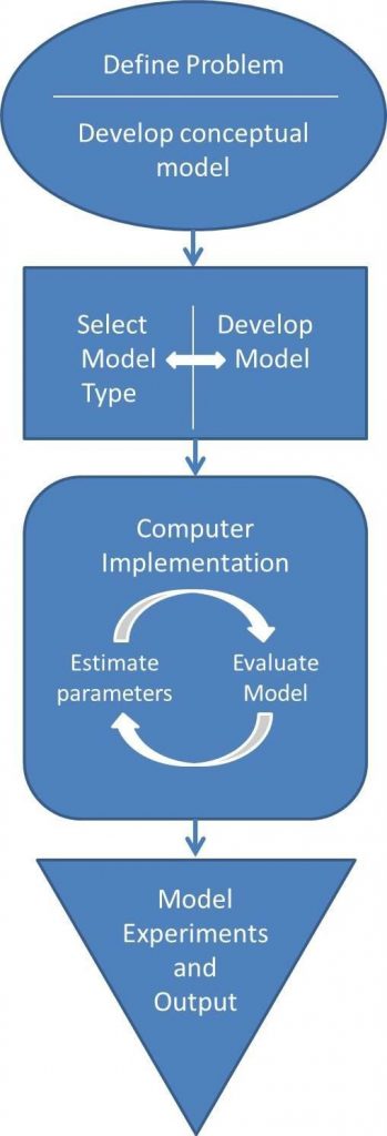
Therefore, the basic steps to model building begin as follows:
- Define the problem
- Develop the conceptual model
- Select the model type – the question and biological processes of focus should drive model selection, discussed next.
- Create model for your system with initial conditions or data.
- Computer implementation
- Parameter estimation
- Model evaluation and iteration
- Experimentation and prediction
Types of Models
Static models describe relationships that are constant and often lack a temporal dimension (time is treated as static). They use empirical data or data derived from expert knowledge to determine or estimate relationships and then apply those relationships more broadly.
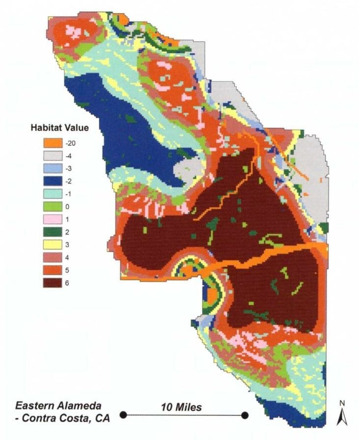
- Habitat and suitability models like those we learned about in earlier lessons are examples of static modeling, such as the model used to map habitat suitability for kit foxes (right).
Dynamic models represent systems or phenomena that change through time. In a dynamic model, there is an interaction (or series of interactions, usually involving movement, growth, etc) associated with each phenomenon in each time step.
- Land cover and land use change models, species dispersal or migration models, and predator/prey models are just some of the dynamic models used in landscape conservation.
In this section, we will expand on our knowledge of static modeling and introduce dynamic modeling.
Static Modeling Process
Static modeling involves several general steps that may be applied through various methodologies:
- Expected relationships between independent and dependent variables are hypothesized; for example between land cover (independent) and fox den selection (dependent).
- When available, empirical data for both independent and dependent variables can inform and validate the model.

Habitat Suitability Modeling
The basic steps of habitat suitability, a static modeling process are:
- Define the goal: every component of the model should relate to the goal
- Establish how to evaluate the model: Each output from a model must be evaluated by objective, measurable criteria to identify the success and usefulness of the model. This should be determined a priori.
- Identify the criteria and attributes that are most important to the biological process: The interaction of these factors should be well understood to build on known mechanisms to expand our knowledge of the system.
- Reclassify the features: It is often important to scale input attributes similarly (e.g. using interval, ratio, or ordinal/rank scales) from most to least preferred/suitable to reflect various model assumptions
- Weight the criteria: Certain criteria are more important than others. Input factors should be weighted consistent with their hypothesized effects
- Combine the reclassified values of all criteria: This will be by simple additional or other mathematical combinations used in weighted overlays
- Analyze the results: The most suitable areas should be identified and verified in the model
- Validate the results: The outcome of the models should be tested with empirical data to determine its success and usefulness
A model scenario: Single-season weighted overlay suitability model for forest elephant in Kenya
In this example, Maasai tribal leaders wish to ensure that elephants migrating from highland forest to lowland habitats during both the wet and dry seasons have enough suitable habitat to sustain the herds and draw tourists.
Model algorithm: each cell location (with raster data) is assigned a value to each attribute or criterion the species is reacting to. The total preference value represents the relative preference of that species for the attributes at that location for all the criteria. The higher the value the more preferred the cell location is assumed to be.
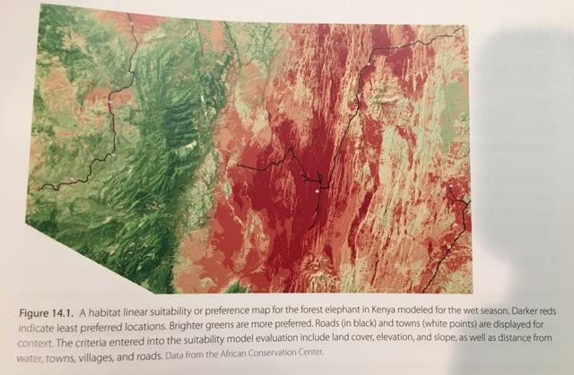
In the resulting map (Figure 14.1), brighter greens are modeled as more preferred habitat for forest elephant in Kenya.
By identifying the best locations for the elephants, the Maasai can also identify other locations to graze their livestock to avoid grazing conflicts with the elephants.
We have previously learned about habitat suitability models in a conceptual manner, however it is important to carefully consider the statistical assumptions and methodologies (e.g. biological preference- assumptions) of a modeling approach before undertaking it.
Maximum Entropy
The Maximum Entropy modeling program uses machine learning to predict the occurrence of organisms based on environmental variables that are predicted to influence their capacity to survive
- This software takes a set of layers or environmental variables as inputs (including elevation, precipitation, etc)
- The software uses georeferenced occurrence locations within sampled areas to estimate relationships.
- The model extrapolates these relationships across the rest of the unsurveyed territory to provide a habitat suitability model.
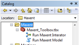
The Maxent toolbox can be utilized through ESRI Arcmap
The user should carefully select input layers expected to influence the species of concern
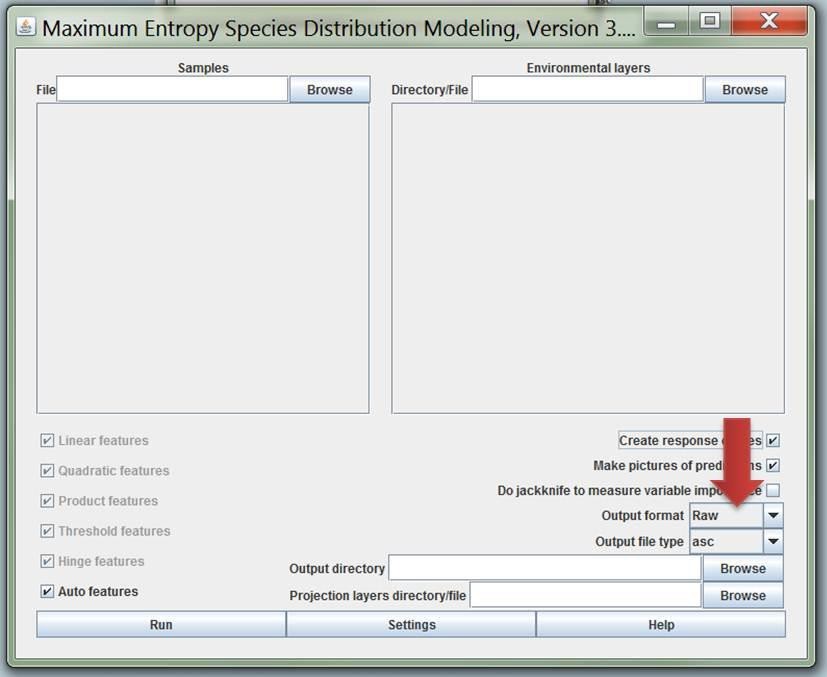
The Maxent outputs extrapolate relationships across the study extent using the relationships defined within the constructed model
 [CC BY 3.0 (https://creativecommons.org/licenses/by/3.0)]")
Dynamic Modeling Process
Dynamic modeling follows a basic process:
- Initial location of the phenomenon is defined
- The time interval for each step is established
- The general movement rules are defined
- The number of time steps to run the model is determined
- The output from one time step is the input for the subsequent time step
- Time and space are explicit and dynamic in the model
There are two kinds of dynamic models.
- Deterministic models represent the average, expected behavior of a system, but lack random variation in the conditions or behavior of the system being modeled. Therefore, a
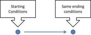 deterministic model will always produce the same output from a given starting condition or initial state.
Algorithm
The input starting conditions and locations of the phenomenon are entered into a series of defined rules. Based on the rules, the phenomenon may change its state and location and may also change the conditions of the landscape and other phenomena that encounter it. The new state and location of the phenomenon and the state and locations of other phenomena are input into the defined rule set.
Assumptions
- The precise outcome can be predicted, because full knowledge of the process and its relationships are understood.
- There is no randomness in the biological process, and all interactions are understood.
- Given the same starting conditions, the output will always be identical.
- The model environment requires feedback and looping capabilities.
- Time is dictated by the modeler’s knowledge of the phenomenon, what aspects of the phenomenon are being modeled, how far the phenomenon can move in a time step, and the resolution of the data.
2. Stochastic models allow for the direct modeling of the random perturbations that underlie real world ecological systems.
Algorithm
This approach is similar to that of deterministic dynamic models but uses random numbers to add stochasticity or randomness. A stream of random numbers are generated and transformed into a distribution, such as uniform, normal, etc. Each distribution captures characteristics of the stochasticity of the biological process. A random number is selected from the distribution. Based on the number selected, the value can be added to existing input data, used to determine what action should or should not be performed, or can alter existing values within a criterion affecting the decision making of the phenomenon.
Assumptions
- The random events in the biological process being modeled can be defined by a specified distribution.
- As with most dynamic models, and more so with dynamic models with stochastic processes, it is virtually impossible to model the precise movement of a phenomenon every time step. Therefore, the models are run many times (called Monte Carlo runs), and the results are combined to create probability surfaces identifying the likelihood of where the phenomenon will be.
- More than likely, each run of the model will produce different results.
Models can also be blended – capturing some processes in a deterministic fashion while simulating the stochasticity of others.
Meet a Landscape Model
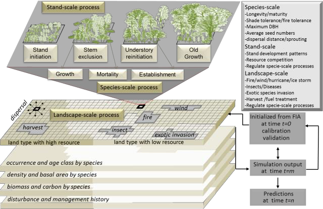
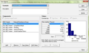 PATH Landscape Model is a dynamic, spatially interactive landscape model designed to project the spatial interactions of vegetation change, natural disturbances, and management at broad spatial scales (up to 250,000 ha) over decades to centuries.
http://essa.com/tools/path-landscape-model/
- In this blended model:
forest communities and successional trajectories are static – species composition and structure are defined a priori for each seral stage and the transition of forest stands between seral stages is defined within a land cover type - the location and size of natural disturbance events are stochastic – a disturbance event such as fire occurs randomly on the landscape and its size can vary (chosen from a distribution)
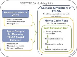 In PATH (or formerly TELSA in figure to right), different variations of spatial and non-spatial inputs can be combined to generate alternative scenarios of natural disturbances and management. Since the model is spatially stochastic, multiple Monte Carlo runs are typically performed for each scenario.
Wise Model Application
“Essentially, all models are wrong, but some are useful.” – George Box
All models are simplifications of reality and cannot possibly capture all of the detailed dynamics and interactions of natural systems. Therefore, models must be carefully and deliberately developed and applied.
Know your model! Performance of any model results from the hypotheses and assumptions on which it is built. Therefore, accurately interpreting and applying the results of a model requires an understanding of how it works, what it considers, and what it does not.
Errors propagate. Understanding the sensitivity of models to error in estimating parameters is critical; however, assessing error propagation in spatial models remains challenging.
Comparing alternative model formulations is extremely valuable.
Technologically advanced methodologies do not assure the accuracy or reliability or results. More complex models do not necessarily decrease the uncertainty of model results.
Scenario Analysis
What is scenario analysis?
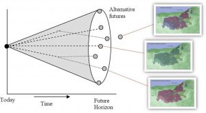
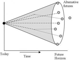 Scenarios are a structured set of stories about alternative futures designed to explore the logical consequences of key uncertainties. Scenario development is a way to explore possibilities for the future that cannot be predicted by extrapolation of past and current trends.
Scenarios provide a tool for integrating different kinds of information (including traditional socio-economic and ecological data, model runs, and perspectives of diverse individuals).
Why do we need scenarios?
Integrated social-ecological dynamics are hard to predict for many reasons. Sometimes we have limited knowledge from the past about a system, or there is high uncertainty in responses to potential change due to a lack of information about socio-ecological dynamics. In addition, past trends cannot always be reliably extrapolated into the future, an important point under changing climate conditions.
Building the scenarios and evaluating their consequences can help the public, decision makers and scientists organize ideas about changes in landscape and regional social-ecological systems.
Millennium Ecosystem Assessment Scenarios
Among the most well-known scenarios are the Millennium Ecosystem Assessment (MEA) scenarios used to explore aspects of plausible global futures and their implications for ecosystem services (Carpenter et al. 2005). The MEA provides the following description of the purpose and details of their scenarios.
The assessment offers policy makers a mechanism to:
- Identify options that can better achieve core human development and sustainability goals. All countries and communities are grappling with the challenge of meeting growing demands for food, clean water, health, and employment.
- Better understand the trade-offs involved—across sectors and stakeholders—in decisions concerning the environment.
- Align response options with the level of governance where they can be most effective.
Purpose of the scenarios
The purpose of the scenarios was to explore the consequences of the four futures for ecosystem services and human well-being. The four futures that were examined were developed based on interviews with leaders in nongovernmental organizations, governments, and business from five continents, on the literature, and on policy documents addressing linkages between ecosystem change and human well-being. No scenario will match the future as it actually occurs. No scenario represents business as usual, though all are based on current conditions and trends. None of the scenarios represents a ‘‘best’’ path or a ‘‘worst’’ path.
Alternative Future Scenarios of Global Change
Four different narrative storylines were developed to explore the plausible future changes in drivers, ecosystems, ecosystem services, and human well-being. Each storyline represents different future demographic, social, economic, technological, and environmental developments. For this reason, their plausibility or feasibility should not be considered solely on the basis of an extrapolation of current economic, technological, and social trends.
 The Global Orchestration scenario depicts a worldwide connected society in which global markets are well developed. Supra-national institutions are well placed to deal with global environmental problems, such as climate change and fisheries. However, their reactive approach to ecosystem management makes them vulnerable to surprises arising from delayed action or unexpected regional changes.
 The Order from Strength scenario represents a regionalized and fragmented world concerned with security and protection, emphasizing primarily regional markets, and paying little attention to the common goods, and with an individualistic attitude toward ecosystem management.
 The Adapting Mosaic scenario depicts a fragmented world resulting from discredited global institutions. It sees the rise of local ecosystem management strategies and the strengthening of local institutions. Investments in human and social capital are geared toward improving knowledge about ecosystem functioning and management, resulting in a better understanding of the importance of resilience, fragility, and local flexibility of ecosystems.
 The TechnoGarden scenario depicts a globally connected world relying strongly on technology and on highly managed and often engineered ecosystems to deliver needed goods and services. Overall, eco- efficiency improves, but it is shadowed by the risks inherent in large-scale human-made solutions. Technology and market-oriented institutional reform are used to achieve solutions.
From Carpenter et al. (2005), Millenium Ecosystem Assessment. Scenarios Working Group
Landscape Scenario Analysis
In regional environmental applications, scenario analysis is often integrated with landscape modeling to create spatially explicit alternative futures resulting from land management, policy, climate change, and resource or energy demand alternatives.
A landscape scenario refers to the different possible conditions that underlie landscape change (Nassauer and Corry 2004), where the alternative futures are spatially explicit representations of plausible landcover patterns (often generated by using landscape modeling).
Scenario-building can also be approached as a collaborative learning process among experts and stakeholders.
Next let’s look at a couple different scenario modeling projects.
Yahara Watershed Scenarios
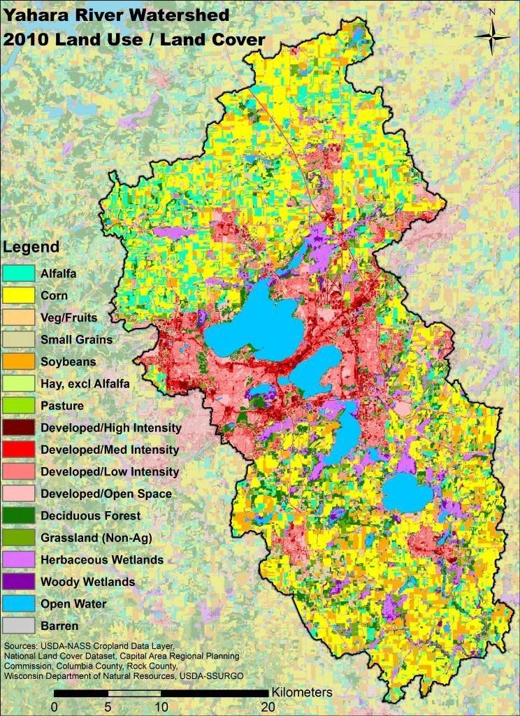
Researchers at UW-Madison developed a set of scenarios of social-ecological change for the Yahara Watershed around Madison, Wisconsin from 2010 to 2070:
- The overarching questions for the scenarios were:
What will be the future condition for human well-being and ecosystem services of the region between the present and 2070? - What human actions will make the region more resilient (or vulnerable) to climate change?
Scenario narratives are accompanied by new modeling studies of climate change, land use and land cover change, hydrology and lake water quality, as well as empirical analyses of governance of natural resources in the watershed.
Click here to explore this project further and learn about how scenario analysis and quantitative modeling are being integrated to answer these questions.
Willamette Valley Alternative Futures Project
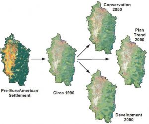
Researchers conducted an alternative futures analysis for the Willamette River Basin in western Oregon, an area home to 68% of Oregon’s population. The Basin also contains the richest native fish fauna in the State and supports several species federally listed as threatened or endangered, including the northern spotted owl and spring Chinook salmon. By 2050, the number of people in the Basin is expected to nearly double, placing tremendous demands on limited resources and creating major challenges for land and water use planning.
Recognizing that conditions of existing landscapes represent a single point on a long-term trajectory of landscape evolution, the study addressed four basic questions:
- how have people altered the land, water and biotic resources over the past 150 years?
- how might human activities alter landscapes over the next 50 years, considering a range of plausible management and policy options?
- what are the expected ecological and socio-economic consequences of these long-term landscape changes? and
- what types of management actions, in what geographic areas or types of ecosystems, are likely to have the greatest effect?
For more information see Baker et al. (2002) Alternative Futures for the Willamette River Basin, Oregon. Ecological Applications 14(2):313–324.
Scenario Modeling
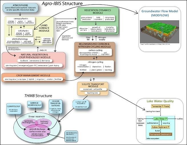
In both of the examples, quantitative modeling is being used to simulate and evaluate the outcomes of the alternative scenarios for each landscape. These quantitative models are integrated as subsets of a larger process. For example, the diagram below shows the family of models being used to evaluate potential future changes in freshwater and related ecosystem services (see table) from present conditions in the Yahara River watershed.
In the next topic, we will explore an example of integrated scenario analysis and modeling to evaluate alternative forest conservation strategies.
Applying landscape scenario modeling
In this topic, we will explore an example of landscape scenario analysis and modeling to evaluate alternative forest conservation strategies from our own research. Chapter 14 in your book highlights several other conservation-based spatial modeling examples using GIS. Please take a look!
Forest Scenarios Project
Aims
The aims of this scenario modeling study were two-fold:
- to enable conservation practitioners and decision-makers to compare the potential outcomes of different conservation strategies and make informed decisions about how to best utilize scarce financial resources and reduce the risks associated with the implementation of innovative strategies.
- to set the stage for continued cooperative conservation planning and adaptive management among the diverse organizations at work on these landscapes.
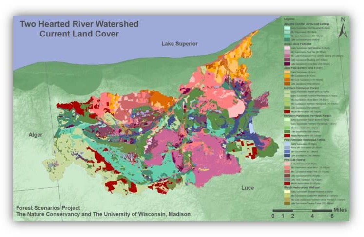
Study Site
The Two Hearted River watershed lies in the eastern portion of Michigan’s Upper Peninsula. It encompasses 53,653 ha of upland hardwood forests, pine stands, and coniferous forests, interspersed with a variety of wetland systems, including muskeg, bogs, and swamps.
 Background: The current ownership and conservation in the watershed are a result of the Northern Great Lakes Forest Project, or the “Big U.P. Deal” as it became known informally – an initiative by The Nature Conservancy (TNC) that began in 2001. Today, the Michigan Department of Natural Resources (DNR), the Forestland Group (a timber investment management organization, or TIMO), and TNC together own 80% of the THR watershed. The remaining 20% is held in private ownerships. All of the land controlled by the TIMO is managed under working forest conservation easements held by the DNR. These diverse owners have multiple management objectives, ranging from a focus on conservation of biodiversity (TNC), improvement of forest condition for investors (TIMOs), and recreation, forest products, and reduction of fire risk (DNR). This area exemplifies the complex mosaic of ownership, management, and conservation challenges typical of broad-scale conservation efforts in the U.S. today.
Scenarios
The Forest Scenarios Project team organized and held workshops with local experts to develop a set of landscape scenarios for the Two Hearted River watershed.
Scenarios were composed of a set of two drivers of landscape change:
- a forest management strategy and
- selected climate change impacts.
Experts identified four management strategies in the THR watershed:
- continuation of current management,
- no conservation action,
- increased area under conservation easement, and
- cooperative ecological forestry.
Click here to explore the details and spatial attributes of these four management scenarios
Experts also identified increased wildfire and windthrow as the climate change impacts of greatest concern in these landscapes. Historically, fire and windthrow were the major disturbances shaping forests of northern Wisconsin and the Upper Peninsula (Schulte and Mladenoff 2005).
Modeling and Analysis
The Forest Scenarios Project team spatially simulated forest ecosystem dynamics in the Two Hearted River watershed for 100 years into the future under each scenario using the TELSA (now PATH) modeling suite described in Topic 1.
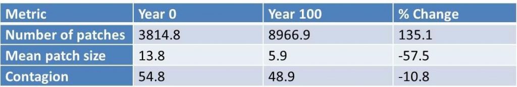
Modeling resulted in land cover maps at 25, 50, 75, and 100 years into the future under each scenario. Landscape metrics were used to quantify change in landscape composition and configuration under each scenario over time. Together, land cover maps and metrics help tell the story of landscape change and enable comparisons between scenarios.
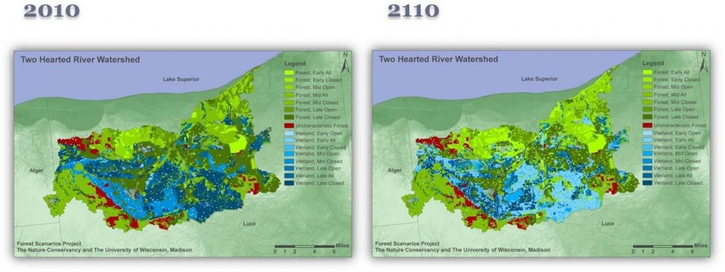
Example Results: Current Management Scenario
Over the course of 100 years, the forests of the THR watershed become younger and more spatially heterogeneous, with mature closed canopy forest and younger, open canopy stands occurring in smaller, interspersed patches.
Land cover modeling and analysis was the first step in further analysis of the changes under each scenario. The results of land cover modeling were used as input for the species habitat modeling. Further analysis also includes evaluation of the ability of the landscape to provision timber and other forest products under each scenario.
Landscape scenario analysis and modeling in this context complements long-term monitoring, enables adjustment of strategies to anticipated future conditions, can inform ongoing and future conservation opportunities and is a useful tool for pre-assessing landscape scale conservation strategies.
Supplemental References:
- Baker et al. (2002) Alternative Futures for the Willamette River Basin, Oregon. Ecological Applications 14(2):313–324.
- Mahmoud M, Liu Y, Hartmann H, Stewart S, Wagener T, Semmens D, Stewart R, Gupta H, Dominguez D, Dominguez F, Hulse D, Letcher R, Rashleigh B, Smith C, Street R, Ticehurst J, Twery M, van Deldenp H, Waldick R, White D, Winter L (2009) A formal framework for scenario development in support of environmental decision-making. Environ Model Softw 24:798–808
- Carpenter, S. R., and Millennium Ecosystem Assessment (Program). Scenarios Working Group. (2005). Ecosystems and human well-being : scenarios : findings of the Scenarios Working Group of the Millennium Ecosystem Assessment, Millennium Ecosystem Assessment series.
Washington, DC: Island Press. - Price, J., J. Silbernagel, N.Miller, R.Swaty, M.White, K.Nixon. (2012). Eliciting expert knowledge to inform landscape modeling of conservation scenarios. EcologicalModeling, http://dx.doi.org/10.1016/j.ecolmodel.2011.09.010.