In this section, we briefly explain what agent-based modeling (ABM) is about, including a paradigmatic example. We also try to clarify the relationship between evolutionary game theory and agent-based modeling, and offer some arguments in favor of implementing evolutionary models using an agent-based approach. Finally, we provide some references to other books that can be used to learn more about how to implement agent-based models.

1. What is agent-based modeling?

Agent-based modeling (ABM) is a methodology used to build formal models of real-world systems that are made up by individual units (such as e.g. atoms, cells, animals, people or institutions) which repeatedly interact among themselves and/or with their environment.

The essence of agent-based modeling

The defining feature of the agent-based modeling approach is that it establishes a direct and explicit correspondence

• between the individual units in the target system to be modeled and the parts of the model that represent these units (i.e. the agents), and also
• between the interactions of the individual units in the target system and the interactions of the corresponding agents in the model (figure 1).

This approach contrasts with e.g. equation-based modeling, where entities of the target system may be represented via average properties or via single representative agents.

Thus, in an agent-based model, the individual units of the system and their repeated interactions are explicitly and individually represented in the model (Edmonds, 2001).^[1] Beyond this, no further assumptions are made in agent-based modeling.

At this point, you may be wondering whether game theory is part of ABM, since in game theory players are indeed explicitly and individually represented in the models.^[2] The key to answer that question is the last sentence in the box above, i.e. “Beyond this, no further assumptions are made in agent-based modeling“. There are certainly many disciplines (e.g. game theory and cellular automata theory) that analyze models where individuals and their interactions are represented explicitly. The key distinction is that these disciplines make further assumptions, i.e. impose additional structure on their models. These additional assumptions constrain the type of models that are analyzed and, by doing so, they often allow for more accurate predictions and/or greater understanding within their (somewhat more limited) scope. Thus, when one encounters a model that fits perfectly into the framework of a particular discipline (e.g. game theory), it seems more appropriate to use the more specific name of the particular discipline, and leave the term “agent-based” for those models which satisfy the defining feature of ABM mentioned above and they do not currently fit in any more specific area of study.

The last sentence in the box also uncovers a key feature of ABM: its flexibility. In principle, you can make your agent-based model as complex as you wish. This has pros and cons. Adding complexity to your model allows you to study any phenomenon you may be interested in, but it also makes analyzing and understanding the model harder (or even sometimes practically impossible) using the most advanced mathematical techniques. Because of this, agent-based models are generally implemented in a programming language and explored using computer simulation. This is so common that the terms agent-based modeling and agent-based simulation are often used interchangeably. The following is a list of some features that traditionally have been difficult to analyze mathematically, and for which agent-based modeling can be useful (Epstein and Axtell, 1996):

• Agents’ heterogeneity. Since agents are explicitly represented in the model, they can be as heterogeneous as the modeler deems appropriate.
• Interdependencies between processes (e.g. demographic, economic, biological, geographical, technological) that have been traditionally studied in different disciplines, and are not often analyzed together. There is no restriction on the type of rules that can be implemented in an agent-based model, so models can include rules that link disparate aspects of the world that are often studied in different disciplines.
• Out-of-equilibrium dynamics. Dynamics are inherent to ABM. Running a simulation consists in applying the rules that define the model over and over, so agent-based models almost invariably include some notion of time within them. Equilibria are never imposed a priori: they may emerge as an outcome of the simulation, or they may not.
• The micro-macro link. ABM is particularly well suited to study how global phenomena emerge from the interactions among individuals, and also how these emergent global phenomena may constrain and shape back individuals’ actions.
• Local interactions and the role of physical space. The fact that agents and their environment are represented explicitly in ABM makes it particularly straightforward and natural to model local interactions (e.g. via networks).

As you can imagine, introducing any of the aspects outlined above in an agent-based model often means that the model becomes mathematically intractable, at least to some extent. However, in this book we will learn that, in many cases, there are various aspects of agent-based models that can be analytically solved, or described using formal approximation results. Our view is that the most useful agent-based models lie at the boundaries of theoretical understanding, and help us push these boundaries. They are advances sufficiently small so that simplified versions of them (or certain aspects of their behaviour) can be fully understood in mathematical terms –thus retaining its analytical rigour–, but they are steps large enough to significantly extend our understanding beyond what is achievable using the most advanced mathematical techniques available.

In my personal (albeit biased) view, the best simulations are those which just peek over the rim of theoretical understanding, displaying mechanisms about which one can still obtain causal intuitions. Probst (1999)

2. What is an agent?

In this book we will use the term agent to refer to a distinct part of our (computational) model that is meant to represent a decision-maker. Agents could represent human beings, non-human animals, institutions, firms, etc. The agents in our models will always play a game, so in this book we will use the term agent and the term player interchangeably.

Agents have individually-owned variables, which describe their internal state (e.g. a strategy), and are able to conduct certain computations or tasks, i.e. they are able to run instructions (e.g. to update their strategy). These instructions are sometimes called decision rules, or rules of behavior, and most often imply some kind of interaction with other agents or with the environment.

The following are some of the individually-owned variables that the agents we are going to implement in this book may have:

• strategy (a number)
• payoff (a number)
• my-coplayers (the set of agents with whom this agent plays the game)
• color (the color of this agent)

And the following are examples of instructions that the agents in most of our models will be able to run:

• to play (play a certain game with my-coplayers and set the payoff appropriately)
• to update-strategy (revise strategy according to a certain decision rule)
• to update-color (set color according to strategy)

3. A paradigmatic example

In this section we present a model that captures the spirit of ABM. The model implements the main features of a family of models proposed by Sakoda (1949, 1971) and –independently– by Schelling (1969, 1971, 1978).^[3][4] Specifically, here we present a computer implementation put forward by Edmonds and Hales (2005).^[5]

In this model there are 133 blue agents and 133 orange agents who live in a 2-dimensional grid made up of 20×20 cells (figure 2). Agents are initially located at random on the grid. The neighborhood of a cell is defined by the eight neighboring cells (i.e. the eight cells which surround it).^[6]

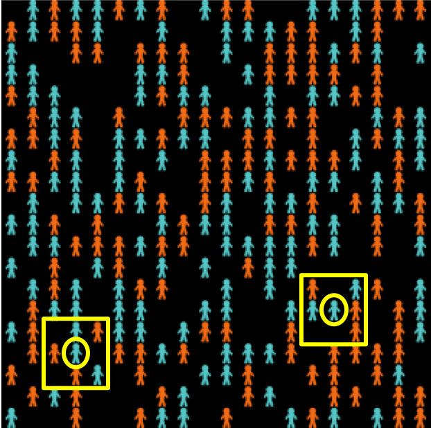
Agents may be happy or unhappy. An agent is happy if the proportion of other agents of its same colour in its neighbourhood is greater or equal than a certain threshold (%-similar-wanted), which is a parameter of the model; otherwise the agent is said to be unhappy. Agents with no neighbors are assumed to be happy regardless of the value of %-similar-wanted. In each iteration of the model one unhappy agent is randomly selected to move to a random empty cell in the lattice.

As an example, the two agents surrounded by a circle in figure 2 have 2 out of 5 neighbors of the same color as them, i.e. 40%. This means that in simulation runs where %-similar-wanted ≤ 40% these agents would be happy, and would not move. On the other hand, in simulations where %-similar-wanted > 40% these two agents would move to a random location.

Now imagine that we simulate a society where agents require at least 60% of their neighbors to be of the same color as them in order to be happy (i.e. %-similar-wanted = 60%). These are pretty strong segregationist preferences, so one would expect a fairly clear pattern of spatial segregation at the end. The following video shows a representative run. You may wish to run the simulations yourself downloading this model’s code.

As expected, the final outcome of the simulation shows clearly distinctive ghettos. To measure the level of segregation of a certain spatial pattern we define a global variable named avg-%similar, which is the average proportion (across agents) of an agent’s neighbors that are the same color as the agent. Extensive Monte Carlo simulation shows that a good estimate of the expected avg-%similar is about 95.7% when %-similar-wanted is 60%.

What is really surprising is that even with only mild segregationist preferences, such as %-similar-wanted = 40%, we still obtain fairly segregated spatial patterns (expected avg-%similar ≈ 82.7%). The following video shows a representative run.

And even with segregationist preferences as weak as %-similar-wanted = 30% (i.e. you are happy unless strictly less than 30% of your neighbors are of the same color as you), the emergent spatial patterns show significant segregation (expected avg-%similar ≈ 74.7%). The following video shows a representative run.

So this agent-based model illustrates how strong spatial segregation can result from only weakly segregationist preferences (e.g. trying to avoid an acute minority status). This model has been enriched in a number of directions (e.g. to include heterogeneity between and within groups),^[7] but the implementation discussed here is sufficient to illustrate a non-trivial phenomenon that emerges from agents’ individual choices and their interactions.

4. Agent-based modeling and evolutionary game theory

Given that models in Evolutionary Game Theory (EGT) comprise many individuals who repeatedly interact among them and occasionally revise their individually-owned strategy, it seems clear that agent-based modelling is certainly an appropriate methodology to build EGT models. Therefore, the question is whether other approaches may be more appropriate or convenient. This is an important issue, since nowadays most models in EGT are equation-based, and therefore –in general– more amenable to mathematical analysis than agent-based models. This is a clear advantage for equation-based models. Why bother with agent-based modeling then?

The reason is that mathematical tractability often comes at a price: equation-based models tend to incorporate several assumptions that are made solely for the purpose of guaranteeing mathematical tractability. Examples include assuming that the population is infinite, or assuming that revising agents are able to evaluate strategies’ expected payoffs. These assumptions are clearly made for mathematical convenience, since there are no infinite populations in the real world, and –in general– it seems more natural to assume that agents’ choices are based on information obtained from experiences with various strategies, or from observations of others’ experiences. Are assumptions made for mathematical convenience harmless? We cannot know unless we study models where such assumptions are not made. And this is where agent-based modelling can play an important role.

Agent-based modeling gives us the potential to build models closer to the real-world systems that we want to study, because in an agent-based model we are free to choose the sort of assumptions that we deem appropriate in purely scientific terms. We may not be able to fully analyze all aspects of the resulting agent-based model mathematically, but we will certainly be able to explore it using computer simulation, and this exploration can help us assess the impact of assumptions that are made only for mathematical tractability. In this way, we will be able to shed light on questions such as: how large must a population be for the mathematical model to be a good description of the dynamics of the finite-population model? and, how much do dynamics change if agents cannot evaluate strategies’ expected payoffs with infinite precision?

5. How can I learn about agent-based modeling?

A wonderful classic book to learn the fundamental concepts and appreciate the kind of models you can build using ABM is Epstein and Axtell (1996). In this short book, the authors show how to build an artificial society where agents, using extremely simple rules, are able to engage in a wide range of activities such as sex, cultural exchange, trade, combat, disease transmission, etc. Epstein and Axtell’s (1996) interdisciplinary book shows how complex patterns can emerge from very simple rules of interaction.

Epstein and Axtell’s (1996) seminal book focuses on the fundamental concepts without discussing any code whatsoever. The following books are also excellent introductions to scientific agent-based modeling, and all of them make use of NetLogo: Gilbert (2007), Railsback and Grimm (2019), Wilensky and Rand (2015) and Janssen (2020). Hamill and Gilbert (2016) discuss the implementation of several NetLogo models in the context of Economics. Most of these models are significantly more sophisticated than the ones we implement and analyze in this book.