
Atomic Orbitals
As was described previously, electrons in atoms can exist only on discrete energy levels but not between them. It is said that the energy of an electron in an atom is quantized, meaning it can be equal only to certain specific values. The electron can jump from one energy level to another, but it cannot transition smoothly because it cannot exist between the levels.
Quantum Numbers
Principal Quantum Number
The energy levels are labeled with an n value, where n = 1, 2, 3, …, ∞. Generally speaking, the energy of an electron in an atom is greater for greater values of n. This number, n, is referred to as the principal quantum number. The principal quantum number defines the location of the energy level. It is essentially the same concept as the n in the Bohr atom description. Another name for the principal quantum number is the shell number.
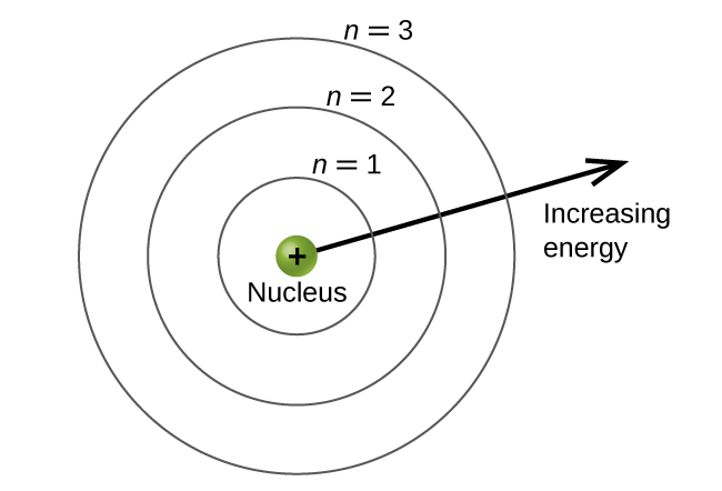
The shells of an atom can be thought of as concentric circles radiating out from the nucleus. The electrons that belong to a specific shell are most likely to be found within the corresponding circular area (not traveling along the circular ring like a planet orbiting the sun). The further we proceed from the nucleus, the higher the shell number, and so the higher the energy level (Figure 1). The positively charged protons in the nucleus stabilize the electronic orbitals by electrostatic attraction between the positive charges of the protons and the negative charges of the electrons. So the further away the electron is from the nucleus, the greater the energy it has.
In a major advance over the Bohr theory of the hydrogen atom, in the quantum mechanical model, one can calculate the quantized energies of any isolated atom. Knowing these energies one can then predict the frequencies and energies of photons that are emitted or absorbed based on the difference of the calculated energy levels using the equation presented in the previous quantum, |ΔE| = |Ef − Ei| = hν. In the case of the hydrogen atom, the expression simplifies to the previously obtained Bohr result.
ΔE = Efinal – Einitial = -2.179 × 10⁻¹⁸  J
J
The principal quantum number is one of three quantum numbers used to characterize an orbital. An atomic orbital, which is distinct from an orbit, is a general region in an atom within which an electron is most probable to reside. More precisely, the orbital specifies the probability of finding an electron in the three-dimensional space around the nucleus and is based on solutions of the Schrödinger equation. In addition, the principal quantum number defines the energy of an electron in a hydrogen or hydrogen-like atom or an ion (an atom or an ion with only one electron) and the general region in which discrete energy levels of electrons in multi-electron atoms and ions are located.
Angular Momentum Quantum Number
Another quantum number is l, the angular momentum quantum number (this is sometimes referred to as the azimuthal quantum number). It is an integer that defines the shape of the orbital, and takes on the values, l = 0, 1, 2, …, n – 1. This means that an orbital with n = 1 can have only one value of l, l = 0, whereas n = 2 permits l = 0 and l = 1, and so on. The principal quantum number defines the general size and energy of the orbital. The l value specifies the shape of the orbital. Orbitals with the same value of l form a subshell.
Magnetic Quantum Number
Angular momentum is a vector. Electrons with angular momentum can have this momentum oriented in different directions. In quantum mechanics it is convenient to describe the z component of the angular momentum. The magnetic quantum number, called ml, specifies the z component of the angular momentum for a particular orbital. For example, if l = 0, then the only possible value of ml is zero. When l = 1, ml can be equal to –1, 0, or +1. Generally speaking, ml can be equal to the set of numbers [–l, –(l –1), …, –1, 0, +1, …, (l – 1), l]. The total number of possible orbitals with the same value of l (a subshell) is 2l + 1. Thus, there is one orbital with l = 0 (ml = 0 is the only orbital), there are three orbitals with l = 1 (ml = -1, ml = 0, ml = 1), five orbitals with l = 2 (ml = -2, ml = -1, ml = 0, ml = 1, ml = 2), and so on.
Rather than specifying all the values of n and l every time we refer to a subshell or an orbital, chemists use an abbreviated system with lowercase letters to denote the value of l for a particular subshell or orbital. Orbitals with l = 0 are called s orbitals (or the s subshell). The value l = 1 corresponds to the p orbitals. For a given n, p orbitals constitute a p subshell (e.g., 3p subshell if n = 3). The orbitals with l = 2 are called the d orbitals, followed by the f, g, and h orbitals for l = 3, 4, 5, and there are higher values we will not consider. When naming a subshell, it is common to write the principal quantum number (n) followed by the subshell letter (s, p, d, f, etc). For example, when referring to a subshell with n = 4 and l = 2, we would call this the 4d subshell. We can also say that there are five different 4d orbitals since there are five values for ml.
As a review, the principal quantum number defines the general value of the electronic energy, with lower values of n indicating lower (more negative) energies and electrons that are closer to the nucleus. The azimuthal quantum number determines the shape of the orbital and we can use s, p, d, f, etc. to designate which subshell the electron is in. And the magnetic quantum number specifies orientation of the orbital in space. Table 1 below provides the possible combinations of n, l, and ml for the first four shells. You’ll notice that every shell does not contain all shapes of orbitals because of the allowable values for the azimuthal quantum number (e.g., there is not a 1p orbital—only shells higher than n = 1 contain a p subshell).
| n | l | Orbital notation | ml | Number of orbitals in a subshell | Number of orbitals in a shell |
| 1 | 0 | 1s | 0 | 1 | 1 |
| 2 | 0 | 2s | 0 | 1 | 4 |
| 1 | 2p | -1, 0, +1 | 3 | ||
| 3 | 0 | 3s | 0 | 1 | 9 |
| 1 | 3p | -1, 0, +1 | 3 | ||
| 2 | 3d | -2, -1, 0, +1, +2 | 5 | ||
| 4 | 0 | 4s | 0 | 1 | 16 |
| 1 | 4p | -1, 0, +1 | 3 | ||
| 2 | 4d | -2, -1, 0, +1, +2 | 5 | ||
| 3 | 4f | -3, -2, -1, 0, +1, +2, +3 | 7 |
Example 1: Working with Shells and Subshells
Indicate the number of subshells, the number of orbitals in each subshell, and the values of l and ml for the orbitals in the n = 4 shell of an atom.
Solution
For n = 4, l can have values of 0, 1, 2, and 3. Thus, four subshells are found in the n = 4 shell of an atom. For l = 0, ml can only be 0. Thus, there is only one orbital with n = 4 and l = 0. For l = 1, ml can have values of –1, 0, +1, so we find three orbitals. For l = 2, ml can have values of –2, –1, 0, +1, +2, so we have five orbitals. When l = 3, ml can have values of –3, –2, –1, 0, +1, +2, +3, and we can have seven orbitals. Thus, we find a total of 16 orbitals in the n = 4 shell of an atom.
Check Your Learning
How many orbitals are in the n = 5 shell?
Answer
25 orbitals
Orbital Shapes
An orbital is the quantum mechanical generalization of Bohr’s orbit. In contrast to his concept of a simple circular orbit with a fixed radius, orbitals are mathematically derived regions of space with different probabilities of having an electron in them.
s-Orbitals
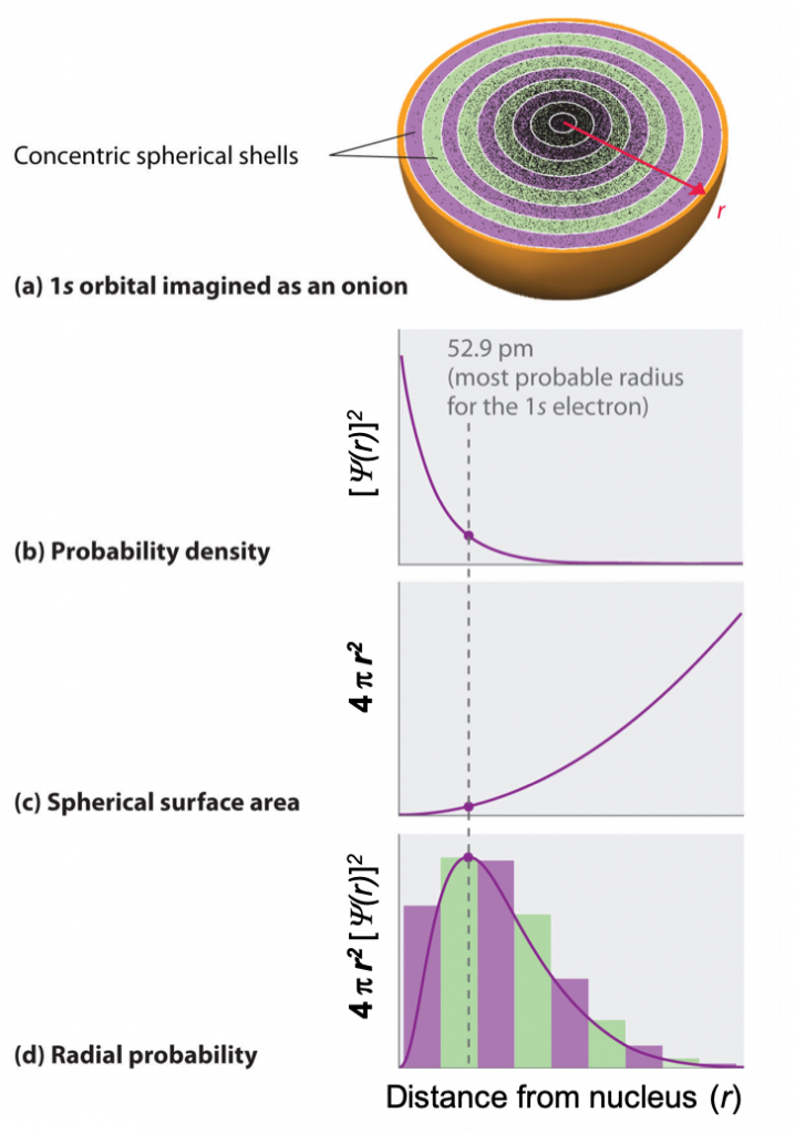
One way of representing electron probability distributions is illustrated in Figure 2 for the 1s orbital of hydrogen. Recall that orbitals are described by wavefunctions, which are represented with ψ. Max Born proposed an interpretation of the wavefunction, ψ, that is still accepted today: the probability density of finding an electron at a given point in space is [ψ(r)]2. In Figure 2a, a dot density diagram is represented. This dot density diagram displays black dots where there is a probability of finding an electron—the higher density of dots, the higher the probability of finding the electron in that region. Taking the information from the dot density diagram, a plot of [ψ(r)]2 versus distance from the nucleus (r) can be constructed. This type of plot (shown in Figure 2b) is a plot of the probability density. This plot shows the probability of finding the electron near a particular point in space that lies a distance r from the nucleus. The 1s orbital is spherically symmetrical, so the probability of finding a 1s electron at any given point depends only on its distance from the nucleus. The probability density is greatest at r = 0 (at the nucleus) and decreases steadily with increasing distance. At very large values of r, the electron probability density is tiny but not exactly zero.
In contrast to the probability density, we can calculate the radial probability (the probability of finding a 1s electron at a distance r from the nucleus) by adding together the probabilities of an electron being at all points on a series of x spherical shells of radius r1, r2, r3,…, rx − 1, rx. In effect, we are dividing the atom into very thin concentric shells, much like the layers of an onion (Figure 2a), and calculating the probability of finding an electron on each spherical shell. Recall that the electron probability density is greatest at r = 0 (Figure 2b), so the density of dots is greatest for the smallest spherical shells in Figure 2a.
The surface area of each spherical shell is equal to 4πr2, which increases rapidly with increasing r (Figure 2c). Because the surface area of the spherical shells increases at first more rapidly with increasing r than the electron probability density decreases, the plot of radial probability has a maximum at a particular distance (Figure 2d). Importantly, when r is very small, the surface area of a spherical shell is so small that the total probability of finding an electron close to the nucleus is very low; at the nucleus, the electron probability vanishes because the surface area of the shell is zero (Figure 2d).
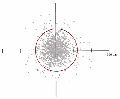
Another representation of the 1s orbital is given in Figure 3. Again, this dot density diagram illustrates the regions where an electron is likely to be found in the “electron cloud”.
A second characteristic evident from Figure 3 is the shape of the electron cloud. In this two-dimensional diagram it appears to be approximately circular; in three dimensions it would be spherical. Figure 4 is a three-dimensional boundary surface diagram for the orbital of the hydrogen atom shown in Figure 3. These boundary surface diagrams are constructed by drawing a circle (or sphere) around a large percentage (say 75 or 90%) of the dots, as has been done in Figure 3 (red line). Since such a sphere or circle encloses most of (but not all) the electron density, it is about as close as one can come to drawing a boundary which describes the shape of the orbital. Boundary surface plots in two and three dimensions are easier to draw quickly than dot-density diagrams, so chemists use them a great deal. Remember that these boundary surface plots are not a specific orbit on which to find an electron (i.e., electrons are not racing around it like a racetrack), but rather a construct to help us visualize where an electron is likely to reside. Therefore, based on Figure 3 and Figure 4, we can say that s orbitals generally have a spherical shape.
Not all s orbitals are the same, however. While the 1s orbital looks like that shown in Figure 4, recall that there are also s orbitals in n = 2, 3, etc. (called 2s, 3s, and ns orbitals). Figure 5 compares the electron probability densities for the hydrogen 1s, 2s, and 3s orbitals. Note that all three are spherically symmetrical. For the 2s and 3s orbitals, however (and for all other s orbitals as well), the electron probability density does not fall off smoothly with increasing r. Instead, a series of minima and maxima are observed in the radial probability plots (Figure 5c). The minima correspond to radial nodes (regions of zero electron probability), which alternate with spherical regions of nonzero electron probability. The orbitals depicted in Figure 5 are of the s type, thus l = 0 for all of them.
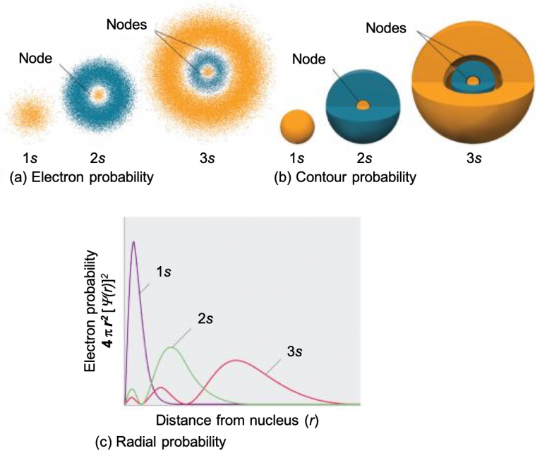
Three things happen to s orbitals as n increases (Figure 5):
- They become larger, extending farther from the nucleus.
- They contain more nodes. This is similar to a standing wave that has regions of significant amplitude separated by nodes (points with zero amplitude). The number of radial nodes in an orbital is n – l – 1.
- For a given atom, the s orbitals also become higher in energy as n increases because of the increased distance from the nucleus.
Orbitals are generally drawn as three-dimensional surfaces that enclose 90% of the electron density. Although such drawings show the relative sizes of the orbitals, they do not normally show the spherical nodes in the 2s and 3s orbitals because the spherical nodes lie inside the 90% surface. Fortunately, the positions of the spherical nodes are not important for chemical bonding. This makes sense because bonding is an interaction of electrons from two atoms, which will be most sensitive to forces at the edges of the orbitals.
p-Orbitals
Only s orbitals are spherically symmetrical. As the value of l increases, the number of orbitals in a given subshell increases, and the shapes of the orbitals become more complex. Because the 2p subshell has l = 1, with three values of ml (−1, 0, and +1), there are three 2p orbitals.
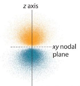
The dot density diagram for one of the hydrogen 2p orbitals is shown in Figure 6. This orbital has two lobes of electron density arranged along the z axis with an electron density of zero in the xy plane. This type of node is called a nodal plane (instead of a radial node which was seen in the s orbitals). Since the xy plane is the nodal plane in Figure 6, it is a 2pz orbital (the orbital is oriented along the z axis).
As shown in Figure 7, the other two 2p orbitals have identical shapes, but they lie along the x axis (2px) and y axis (2py), respectively. Note that each 2p orbital has just one nodal plane.
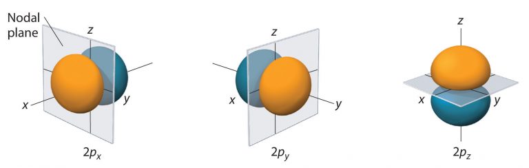
Just as with the s orbitals, the size and complexity of the p orbitals for any atom increase as the principal quantum number n increases. The shapes of the 90% probability surfaces of the 3p, 4p, and higher-energy p orbitals are, however, essentially the same as those shown in Figure 7. The shapes of p orbitals for n > 2 look like strings of beads oriented along the x, y, and z axis with two additional nodes per unit increases in n.
d-Orbitals
Subshells with l = 2 have five d orbitals; the first shell to have a d subshell corresponds to n = 3. The five d orbitals have ml values of −2, −1, 0, +1, and +2.
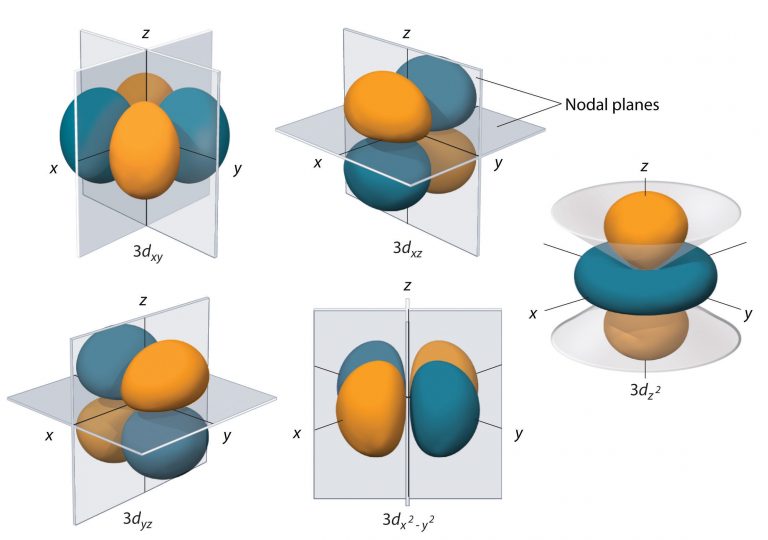
The hydrogen 3d orbitals, shown in Figure 8, have more complex shapes than the 2p orbitals. All five 3d orbitals contain two nodal planes, as compared to one for each p orbital and zero for each s orbital. In three of the d orbitals, the lobes of electron density are oriented between the x and y, x and z, and y and z planes; these orbitals are referred to as the 3dxy, 3dxz, and 3dyz orbitals, respectively. A fourth d orbital has lobes lying along the x and y axes; this is the 3dx2-y2 orbital. The fifth 3d orbital, called the 3dz2 orbital, has a unique shape: it looks like a 2pz orbital combined with an additional doughnut of electron probability lying in the xy plane. Despite its peculiar shape, the 3dz2 orbital is mathematically equivalent to the other four and has the same energy. Like the s and p orbitals, as n increases, the size of the d orbitals increases, but the overall shapes remain similar to those depicted in Figure 8.
f-Orbitals
Principal shells with n = 4 can have subshells with l = 3 and ml values of −3, −2, −1, 0, +1, +2, and +3. These subshells consist of seven f orbitals. Although these orbitals play an important role in the heavier elements, their shapes are complicated and we will not consider these shapes in this course
