
Orbital Energies, Spin, and Electron Configurations
Spin Quantum Number
It was demonstrated in the 1920s that when hydrogen line spectra are examined at extremely high resolution, some lines are actually not single peaks but rather pairs of closely spaced lines. This is the so-called fine structure of the spectrum, and it implies that there are additional small differences in energies of electrons even when they are located in the same orbital. These observations led Samuel Goudsmit and George Uhlenbeck to propose that electrons have a fourth quantum number. They called this the spin quantum number, or ms.
The other three quantum numbers—n, l, and ml—are properties of specific atomic orbitals that define the most likely location in space of an electron. These orbitals are a result of solving the Schrödinger equation for electrons in atoms. The electron spin is a different kind of property. It is a completely quantum phenomenon with no analogues in the classical realm. In addition, it cannot be derived from solving the Schrödinger equation and is not related to the normal spatial coordinates (such as the Cartesian x, y, and z). Electron spin describes an intrinsic electron “rotation” or “spinning.” Each electron acts as a tiny magnet, just as if it were a tiny rotating object charged with an angular momentum, even though this rotation cannot be observed in terms of the spatial coordinates.
The magnitude of the overall electron spin can only have one value, and an electron can only “spin” in one of two quantized states. One is termed the α state, with the z component of the spin being in the positive direction of the z axis. This corresponds to the spin quantum number ms = +½. The other is called the β state, with the z component of the spin being negative and ms = -½. Any electron, regardless of the atomic orbital it is located in, can only have one of those two values of the spin quantum number. The energies of electrons having ms = -½ and ms = ½ are different if an external magnetic field is applied.
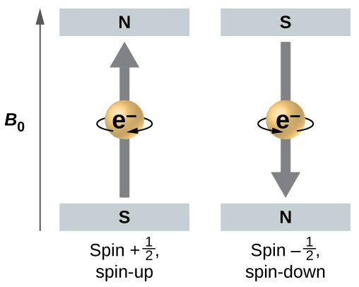
Figure 1 illustrates this phenomenon. An electron acts like a tiny magnet. Its moment is directed up (in the positive direction of the z axis) for the +½ spin quantum number and down (in the negative z direction) for the -½ spin quantum number. A magnet has a lower energy if its magnetic moment is aligned with the external magnetic field (the left electron in Figure 1) and a higher energy for the magnetic moment being opposite to the applied field. This is why an electron with ms = +½ has a slightly lower energy in an external field in the positive z direction, and an electron with ms = -½ has a slightly higher energy in the same field. This is true even for an electron occupying the same orbital in an atom. A spectral line corresponding to a transition for electrons between the same orbitals but with different spin quantum numbers has two possible values of energy; thus, the line in the spectrum will show a fine structure splitting.
The Pauli Exclusion Principle
An electron in an atom is completely described by four quantum numbers: n, l, ml, and ms. The first three quantum numbers define the orbital and the fourth quantum number describes the intrinsic electron property called spin. An Austrian physicist Wolfgang Pauli formulated a general principle that gives the last piece of information that we need to understand the general behavior of electrons in atoms. The Pauli exclusion principle can be formulated as follows: No two electrons in the same atom can have exactly the same set of all four quantum numbers. What this means is that electrons can share the same orbital (the same set of the quantum numbers n, l, and ml), but only if their spin quantum numbers, ms, have different values. Since the spin quantum number can only have two values (± ½), no more than two electrons can occupy the same orbital (and if two electrons are located in the same orbital, they must have opposite spins). Therefore, any atomic orbital can be populated by only zero, one, or two electrons.
The properties and meaning of the quantum numbers of electrons in atoms are briefly summarized in Table 1.
| Name | Symbol | Allowed values | Physical meaning |
| principal quantum number | n | 1, 2, 3, 4, …. | shell, the general region of an electron in the orbital (distance away from the nucleus) |
| azimuthal (or angular momentum) quantum number | l | 0 ≤ l ≤ n–1 | subshell, the shape of the orbital |
| magnetic quantum number | ml | – l ≤ ml ≤ l | orientation of the orbital |
| spin quantum number | ms | +½, −½ | direction of the intrinsic quantum “spinning” of the electron |
Example 1: Maximum Number of Electrons
Calculate the maximum number of electrons that can occupy a shell with (a) n = 2, (b) n = 5, and (c) n as a variable. Note you are only looking at the orbitals with the specified n value, not those at lower energies.
Solution
(a) When n = 2, there are four orbitals (a single orbital with l = 0, and three orbitals labeled l = 1). These four orbitals can contain eight electrons.
(b) When n = 5, there are five subshells of orbitals that we need to sum:
1 orbital with l = 0
3 orbitals with l = 1
5 orbitals with l = 2
7 orbitals with l = 3
+ 9 orbitals with l = 4
———————————————
25 orbitals total
Again, each orbital holds two electrons, so 50 electrons can fit in this shell.
(c) The number of orbitals in any shell n will equal n2. There can be up to two electrons in each orbital, so the maximum number of electrons will be 2 × n2
Check Your Learning
If a shell contains a maximum of 32 electrons, what is the principal quantum number, n?
Answer
n = 4
Orbital Energies
Single Electron
Although we have discussed the shapes of orbitals, we have said little about their comparative energies. We begin our discussion of orbital energies by considering atoms or ions with only a single electron (such as H or He+). This is the simplest case.
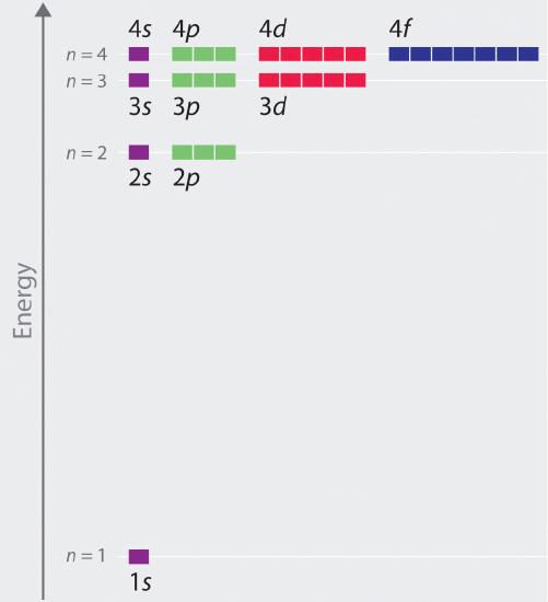
The relative energies of the atomic orbitals with n ≤ 4 for a hydrogen atom are plotted in Figure 2. Note that the orbital energies depend on only the principal quantum number n, not on l. Consequently, the energies of the 2s and 2p orbitals of hydrogen are the same; the energies of the 3s, 3p, and 3d orbitals are the same; and so forth. The orbital energies obtained for hydrogen using quantum mechanics are exactly the same as the allowed energies calculated by Bohr. In contrast to Bohr’s model, however, which allowed only one orbit for each energy level, quantum mechanics predicts that there are 4 orbitals with different electron density distributions in the n = 2 principal shell (one 2s and three 2p orbitals), 9 in the n = 3 principal shell, and 16 in the n = 4 principal shell. As we have just seen, quantum mechanics predicts that in the hydrogen atom, all orbitals with the same value of n (e.g., the three 2p orbitals) are degenerate, meaning that they have the same energy. Figure 2 shows that the energy levels become closer and closer together as the value of n increases, as expected because of the 1/n2 dependence of orbital energies.
Two or More Electrons
The energy of atomic orbitals increases as the principal quantum number, n, increases. In any atom with two or more electrons, the repulsion between the electrons makes energies of subshells with different values of l differ so that the energy of the orbitals increases within a shell in the order s < p < d < f. Figure 3 depicts the trends of increasing energy with increasing n and increasing l (note that this is different than the orbital diagram for hydrogen in Figure 2 because now we have more than one electron).
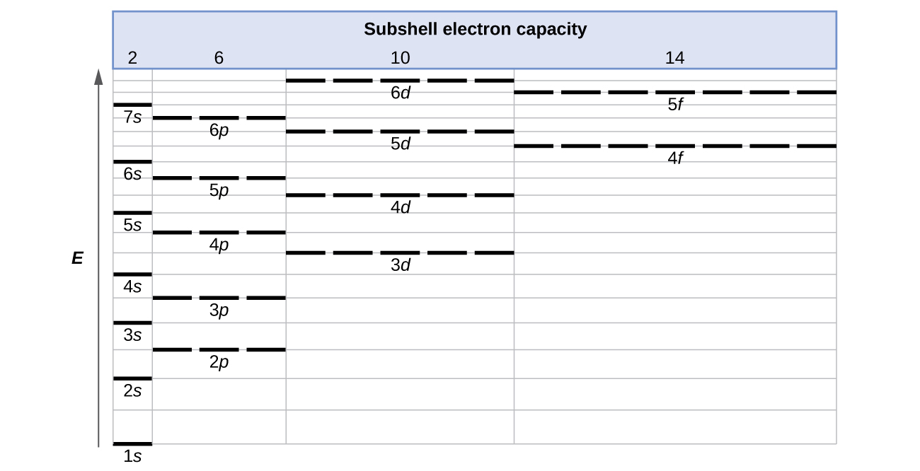
The 1s orbital at the bottom of Figure 3 is the orbital with electrons of lowest energy. The energy increases as we move up to the 2s and then 2p, 3s, and 3p orbitals, showing that the increasing n value has more influence on energy than the increasing l value for small atoms. However, this pattern does not hold for larger atoms. For example, the 3d orbital is higher in energy than the 4s orbital. Such overlaps continue to occur frequently as we move up the chart.
Electrons in successive atoms on the periodic table tend to fill low-energy orbitals first. Thus, many students find it confusing that, for example, the 5p orbitals fill immediately after the 4d, and immediately before the 6s. The filling order is based on observed experimental results, and has been confirmed by theoretical calculations. As the principal quantum number, n, increases, the size of the orbital increases and the electrons spend more time farther from the nucleus. Thus, the attraction to the nucleus is weaker and the energy associated with the orbital is higher (less stabilized). But this is not the only effect we have to take into account. Within each shell, as the value of l increases, the electrons are less penetrating (meaning there is less electron density found close to the nucleus), in the order s > p > d > f. Electrons that are closer to the nucleus slightly repel electrons that are farther out, offsetting the more dominant electron–nucleus attractions slightly (recall that all electrons have −1 charges, but nuclei have +Z charges).
This phenomenon is called shielding and will be discussed in more detail later. Electrons in orbitals that experience more shielding are less stabilized and thus higher in energy. For small orbitals (1s through 3p), the increase in energy due to n is more significant than the increase due to l; however, for larger orbitals the two trends are comparable and cannot be simply predicted.
Electron Configurations of Atoms
The arrangement of electrons in the orbitals of an atom is called the electron configuration of the atom. We describe an electron configuration with a symbol that contains three pieces of information (Figure 4):
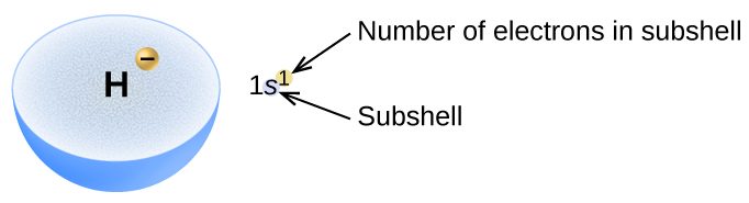
- The number of the principal quantum number, n,
- The letter that designates the orbital type (the subshell, l), and
- A superscript number that designates the number of electrons in that particular subshell.
For example, 2p4 indicates four electrons in a p subshell (l = 1) with a principal quantum number (n) of 2. The notation 3d8 (read “three–d–eight”) indicates eight electrons in the d subshell (l = 2) of the principal shell for which n = 3.
The Aufbau Principle
To determine the electron configuration for any particular atom, we can “build” the structures in the order of atomic numbers. Beginning with hydrogen, and continuing across the periods of the periodic table, we add one proton at a time to the nucleus and one electron to the proper subshell until we have described the electron configurations of all the elements. This procedure is called the Aufbau principle, from the German word Aufbau (“to build up”). Each added electron occupies the subshell of lowest energy available (in the order shown in Figure 3), subject to the limitations imposed by the allowed quantum numbers according to the Pauli exclusion principle. Electrons enter higher-energy subshells only after lower-energy subshells have been filled to capacity.
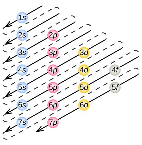
Figure 5 illustrates the traditional way to remember the filling order for atomic orbitals.
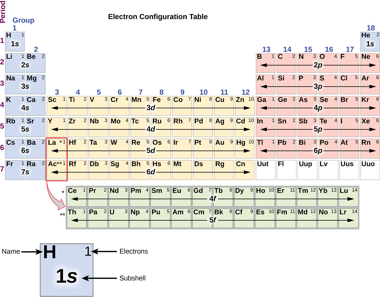
Since the arrangement of the periodic table is based on the electron configurations, Figure 6 provides an alternative method for determining the electron configuration. The filling order simply begins at hydrogen and includes each subshell as you proceed in increasing Z order. For example, after filling the 3p block up to Ar, we see the orbital will be 4s (K, Ca), followed by the 3d orbitals.
Writing Orbital Diagrams
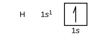
We will now construct the ground-state electron configuration and orbital diagram for a selection of atoms in the first and second periods of the periodic table. Orbital diagrams are pictorial representations of the electron configuration, showing the individual orbitals and the pairing arrangement of electrons. We start with a single hydrogen atom (atomic number 1), which consists of one proton and one electron. Referring to Figure 5 or Figure 6, we would expect to find the electron in the 1s orbital. By convention, the ms = +½ value is usually filled first. The electron configuration and the orbital diagram are:
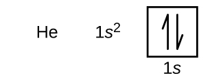
Following hydrogen is the noble gas helium, which has an atomic number of 2. The helium atom contains two protons and two electrons. The first electron has the same four quantum numbers as the hydrogen atom electron (n = 1, l = 0, ml = 0, ms = +½). The second electron also goes into the 1s orbital and fills that orbital. The second electron has the same n, l, and ml quantum numbers, but must have the opposite spin quantum number, ms = -½. This is in accord with the Pauli exclusion principle: No two electrons in the same atom can have the same set of four quantum numbers. For orbital diagrams, this means two arrows go in each box (representing two electrons in each orbital) and the arrows must point in opposite directions (representing paired spins). The electron configuration and orbital diagram of helium are:
The n = 1 shell is completely filled in a helium atom.
The next atom is the alkali metal lithium with an atomic number of 3. The first two electrons in lithium fill the 1s orbital and have the same sets of four quantum numbers as the two electrons in helium. The remaining electron must occupy the orbital of next lowest energy, the 2s orbital. Thus, the electron configuration and orbital diagram of lithium are:

An atom of the alkaline earth metal beryllium, with an atomic number of 4, contains four protons in the nucleus and four electrons surrounding the nucleus. The fourth electron fills the remaining space in the 2s orbital.

An atom of boron (atomic number 5) contains five electrons. The n = 1 shell is filled with two electrons and three electrons will occupy the n = 2 shell. Because any s subshell can contain only two electrons, the fifth electron must occupy the next energy level, which will be a 2p orbital. There are three degenerate 2p orbitals (ml = −1, 0, +1) and the electron can occupy any one of these p orbitals. When drawing orbital diagrams, we include empty boxes to depict any empty orbitals in the same subshell that we are filling.
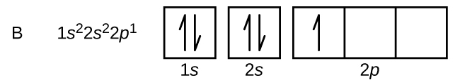
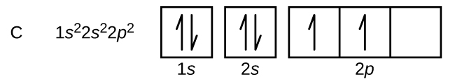
Carbon (atomic number 6) has six electrons. Four of them fill the 1s and 2s orbitals. The remaining two electrons occupy the 2p subshell. We now have a choice of filling one of the 2p orbitals and pairing the electrons or of leaving the electrons unpaired in two different, but degenerate, p orbitals. The orbitals are filled as described by Hund’s rule: The lowest-energy configuration for an atom with electrons within a set of degenerate orbitals is that having the maximum number of unpaired electrons with parallel spins. Placing the electrons in different orbitals and with parallel spins tends to keep the electrons in different regions of space, thus minimizing their Coulomb repulsion and lowering the energy. Thus, the two electrons in the carbon 2p orbitals have identical n, l, and ms quantum numbers and differ in their ml quantum number (in accord with the Pauli exclusion principle). The electron configuration and orbital diagram for carbon are:
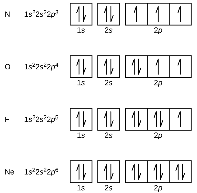
Nitrogen (atomic number 7) fills the 1s and 2s subshells and has one electron in each of the three 2p orbitals, in accordance with Hund’s rule. These three electrons have unpaired spins. Oxygen (atomic number 8) has a pair of electrons in any one of the 2p orbitals (the electrons have opposite spins) and a single electron in each of the other two. Fluorine (atomic number 9) has only one 2p orbital containing an unpaired electron. All of the electrons in the noble gas neon (atomic number 10) are paired, and all of the orbitals in the n = 1 and the n = 2 shells are filled. The electron configurations and orbital diagrams of these four elements are:
The alkali metal sodium (atomic number 11) has one more electron than the neon atom. This electron must go into the lowest-energy subshell available, the 3s orbital, giving a 1s22s22p63s1 configuration. We can abbreviate electron configurations by writing the a noble gas configuration, which consists of the elemental symbol of the last noble gas prior to that atom, followed by the configuration of the remaining electrons. For our sodium example, the noble gas (or abbreviated or condensed) configuration is [Ne]3s1.
When we come to the alkali metal potassium (atomic number 19), we might expect that we would begin to add electrons to the 3d subshell. However, all available chemical and physical evidence indicates that potassium is like lithium and sodium, and that the next electron is not added to the 3d level but is, instead, added to the 4s level. As discussed previously, the 3d orbital with no radial nodes is higher in energy because it is less penetrating and more shielded from the nucleus than the 4s, which has three radial nodes. Thus, potassium has an electron configuration of [Ar]4s1.
Beginning with the transition metal scandium (atomic number 21), additional electrons are added successively to the 3d subshell. This subshell is filled to its capacity with 10 electrons (remember that for l = 2 [d orbitals], there are 2l + 1 = 5 values of ml, meaning that there are five d orbitals that have a combined capacity of 10 electrons). The 4p subshell fills next. Note that for three series of elements, scandium (Sc) through copper (Cu), yttrium (Y) through silver (Ag), and lutetium (Lu) through gold (Au), a total of 10 d electrons are successively added to the (n – 1) shell next to the n shell to bring that (n – 1) shell from 8 to 18 electrons. For two series, lanthanum (La) through lutetium (Lu) and actinium (Ac) through lawrencium (Lr), 14 f electrons (l = 3, 2l + 1 = 7 ml values; thus, seven orbitals with a combined capacity of 14 electrons) are successively added to the (n – 2) shell to bring that shell from 18 electrons to a total of 32 electrons.
Example 2: Quantum Numbers and Electron Configurations
What is the electron configuration and orbital diagram for a phosphorus atom? What are the four quantum numbers for the last electron added?
Solution
The atomic number of phosphorus is 15. Thus, a phosphorus atom contains 15 electrons. The order of filling of the energy levels is 1s, 2s, 2p, 3s, 3p, 4s, . . . The 15 electrons of the phosphorus atom will fill up to the 3p orbital, which will contain three electrons:
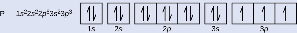
The last electron added is a 3p electron. Therefore, n = 3 and, for a p-type orbital, l = 1. The ml value could be –1, 0, or +1. The three p orbitals are degenerate, so any of these ml values is correct. For unpaired electrons, convention assigns the value of +½ for the spin quantum number; thus, ms = +½.
Check Your Learning
Identify the atoms from the electron configurations given:
- [Ar]4s23d5
- [Kr]5s24d105p6
Answer
(a) Mn; (b) Xe
Electron Configuration Exceptions
The periodic table can be a powerful tool in predicting the electron configuration of an element. However, we do find exceptions to the order of filling of orbitals shown in Figure 6. For instance, the ground state electron configuration of the transition metal chromium (Cr; atomic number 24) is [Ar]4s13d5 and that of copper (Cu; atomic number 29) is [Ar]4s13d10. In general, such exceptions involve subshells with very similar energy, and small effects can lead to changes in the order of filling.
In the case of Cr and Cu, we find that half-filled and completely filled subshells apparently represent conditions of preferred stability. This stability is such that an electron shifts from the 4s into the 3d orbital to gain the extra stability of a half-filled 3d subshell (in Cr) or a filled 3d subshell (in Cu). Other exceptions also occur. For example, niobium (Nb, atomic number 41) is predicted to have the electron configuration [Kr]5s24d3. Experimentally, we observe that its ground-state electron configuration is actually [Kr]5s14d4. We can rationalize this observation by saying that the electron–electron repulsions experienced by pairing the electrons in the 5s orbital are larger than the gap in energy between the 5s and 4d orbitals. There is no simple method to predict the exceptions for atoms where the magnitude of the repulsions between electrons is greater than the small differences in energy between subshells.
