
Wave-Particle Duality
Wave Interference and Diffraction

If you were to drop a stone into a still pond, you would see waves ripple outward from the center of a circle. If you were to drop multiple stones into a still pond, you would see these same waves ripple outward, but when the waves meet, the pattern would change. When two or more waves come into contact, they interfere with each other. Interacting waves on the surface of water can produce interference patterns similar to those shown below (Figure 1).
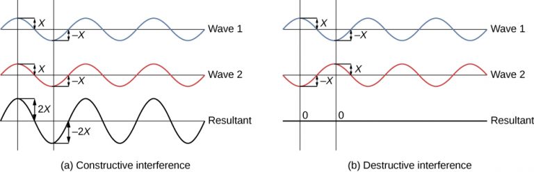
There are two types of wave interference. Constructive interference occurs in regions where the peaks or troughs for the two waves coincide (Figure 2a). Destructive interference occurs in regions where the peak of one wave coincides with the trough of another wave (Figure 2b). The amplitudes of the interfering waves add together and produce a resultant wave, as shown below.

Diffraction of waves occurs when a wave encounters an obstacle—the wave appears to bend around a small obstacle or spread out in semicircles after an opening. Consider the water waves in Figure 3 that show how water waves diffract and form large semicircles after passing through a breakwater.
Light Behaves as a Wave
The interference that is seen in water waves is also seen with light, which indicates that light behaves like a wave. Figure 4 shows the interference patterns that arise when light passes through narrow slits closely spaced about a wavelength apart. If light behaved as a classic particle, shining a light through two narrowly spaced slits would result in just two lines on the screen (one for the light particles passing through each slit). The fact that an interference pattern occurs indicates that a pure particle definition of light is not accurate.

The fringe patterns produced depend on the wavelength. If you were to pass short and long wavelength light through a set of slits, the shorter wavelength light will produce more closely spaced fringes than longer wavelength light. When the light passes through the two slits, each slit effectively acts as a new source, resulting in two closely spaced waves coming into contact at the detector (the camera in this case). The dark regions in Figure 4 correspond to regions where the peaks for the wave from one slit happen to coincide with the troughs for the wave from the other slit (destructive interference), while the brightest regions correspond to the regions where the peaks for the two waves (or their two troughs) happen to coincide (constructive interference). Such interference patterns cannot be explained by particles moving according to the laws of classical mechanics.

If light passes through a slit, it will also produce a similar wave pattern as depicted in Figure 3. A wave passing through two small openings spaced closely together will spread out and begin to interfere, as seen in Figure 5. A wave comes from the left and is incident on two slits, which diffract the plane wave. The interference pattern produced when light diffracts cannot be explained by particles moving according to the laws of classical mechanics.
Since the photoelectric effect showed that light has particle-like characteristics, and light diffraction and interferences shows that light has wave-like properties, we often refer to the wave-particle duality of light: Light has both wave-like and particle-like properties.
Behavior in the Microscopic World and De Broglie Wavelength
We know how matter behaves in the macroscopic world—objects that are large enough to be seen by the naked eye follow the rules of classical physics. A billiard ball moving on a table will behave like a particle: It will continue in a straight line unless it collides with another ball or the table cushion, or is acted on by some other force (such as friction). The ball has a well-defined position and velocity (or a well-defined momentum, p = mv, defined by mass m and velocity v) at any given moment. In other words, the ball is moving in a classical trajectory. This is the typical behavior of a classical object.
One of the first people to pay attention to the special behavior of the microscopic world was Louis de Broglie. He asked the question: If electromagnetic radiation can have particle-like character, can electrons and other submicroscopic particles exhibit wavelike character? In his 1925 doctoral dissertation, de Broglie extended the wave–particle duality of light that Einstein used to resolve the photoelectric effect paradox to material particles. He predicted that a particle with mass m and velocity v (that is, with linear momentum p) should also exhibit the behavior of a wave with a wavelength value λ, given by this expression in which h is the familiar Planck’s constant:
λ = 
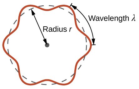
This quantity is called the de Broglie wavelength. Unlike the other values of λ discussed thus far, the de Broglie wavelength is a characteristic of particles and other bodies, not electromagnetic radiation (note that this equation involves velocity [v, with units m/s], not frequency [ν, with units Hz]. Although these two symbols are similar, they mean very different things). Where Bohr had postulated the electron as being a particle orbiting the nucleus in quantized orbits, de Broglie argued that Bohr’s assumption of quantization can be explained if the electron is considered not as a particle, but rather as a circular standing wave such that only an integer number of wavelengths could fit exactly within the orbit (Figure 6).
Interference Patterns are a Hallmark of Wavelike Behavior
Shortly after de Broglie proposed the wave nature of matter, two scientists at Bell Laboratories, C. J. Davisson and L. H. Germer, demonstrated experimentally that electrons can exhibit wavelike behavior by showing an interference pattern for electrons reflecting off a crystal. The same interference pattern is also observed when electrons travel through a regular atomic pattern in a crystal. The regularly spaced atomic layers served as slits that diffract the electrons, as used in other interference experiments. Since the spacing between the layers serving as slits needs to be similar in size to the wavelength of the tested wave for an interference pattern to form, Davisson and Germer used a crystalline nickel target for their “slits,” since the spacing of the atoms within the lattice was approximately the same as the de Broglie wavelengths of the electrons that they used.
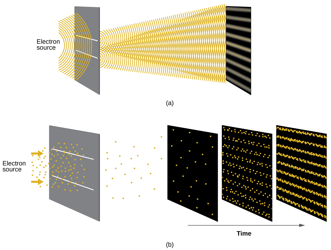
Figure 7 shows an interference pattern. The wave–particle duality of matter can be seen in Figure 7 by observing what happens if electron collisions are recorded over a long period of time. Initially, when only a few electrons have been recorded, they show clear particle-like behavior, having arrived in small localized packets that appear to be random. As more and more electrons arrived and were recorded, a clear interference pattern that is the hallmark of wavelike behavior emerged. Thus, it appears that while electrons are small localized particles, their motion does not follow the equations of motion implied by classical mechanics, but instead it is governed by some type of a wave equation that governs a probability distribution even for a single electron’s motion. Thus the wave–particle duality first observed with photons is actually a fundamental behavior intrinsic to all quantum particles.
Chemistry in Real Life: Dorothy Hodgkin
Because the wavelengths of X-rays (10-10,000 picometers [pm]) are comparable to the size of atoms, X-rays can be used to determine the structure of molecules. When a beam of X-rays is passed through molecules packed together in a crystal, the X-rays collide with the electrons and scatter. Constructive and destructive interference of these scattered X-rays creates a specific diffraction pattern. Calculating backward from this pattern, the positions of each of the atoms in the molecule can be determined very precisely. One of the pioneers who helped create this technology was Dorothy Crowfoot Hodgkin.
She was born in Cairo, Egypt, in 1910, where her British parents were studying archeology. Even as a young girl, she was fascinated with minerals and crystals. When she was a student at Oxford University, she began researching how X-ray crystallography could be used to determine the structure of biomolecules. She invented new techniques that allowed her and her students to determine the structures of vitamin B12, penicillin, and many other important molecules. Diabetes, a disease that affects 382 million people worldwide, involves the hormone insulin. Hodgkin began studying the structure of insulin in 1934, but it required several decades of advances in the field before she finally reported the structure in 1969. Understanding the structure has led to better understanding of the disease and treatment options.
Example 1: Calculating the Wavelength of a Particle
If an electron travels at a velocity of 1.000 × 10⁷ m/s and has a mass of 9.109 × 10⁻²⁸ g, what is its wavelength?
Solution
We can use de Broglie’s equation to solve this problem, but we first must do a unit conversion of Planck’s constant. You learned earlier that 1 J = 1 kg·m2/s2. Thus, we can write h = 6.626 × 10⁻³⁴ J·s as 6.626 × 10⁻³⁴ kg·m2/s.
λ =  = 7.274 × 10⁻¹¹ m
This is a small value, but it is significantly larger than the size of an electron in the classical (particle) view. This size is the same order of magnitude as the size of an atom. This means that electron wavelike behavior is going to be noticeable in an atom.
Check Your Learning
Calculate the wavelength of a softball with a mass of 100 g traveling at a velocity of 35 m/s, assuming that it can be modeled as a single particle.
Answer
1.9 × 10⁻³⁴ m
We never think of a thrown softball having a wavelength, since this wavelength is so small it is impossible for our senses or any known instrument to detect. The de Broglie wavelength is only appreciable for matter that has a very small mass and/or a very high velocity.
The Quantum–Mechanical Model of an Atom
Shortly after de Broglie published his ideas that the electron in a hydrogen atom could be better thought of as being a circular standing wave instead of a particle moving in quantized circular orbits, as Bohr had argued, Erwin Schrödinger extended de Broglie’s work by incorporating the de Broglie relation into a wave equation, deriving what is today known as the Schrödinger equation. When Schrödinger applied his equation to hydrogen-like atoms, he was able to reproduce Bohr’s expression for the energy and, thus, the Rydberg formula governing hydrogen spectra. He did so without having to invoke Bohr’s assumptions of stationary states and quantized orbits, angular momenta, and energies. Quantization in Schrödinger’s theory was a natural consequence of the underlying mathematics of the wave equation. Like de Broglie, Schrödinger initially viewed the electron in hydrogen as being a physical wave instead of a particle, but where de Broglie thought of the electron in terms of circular stationary waves, Schrödinger properly thought in terms of three-dimensional stationary waves, or wavefunctions, represented by the Greek letter psi, ψ. A few years later, Max Born proposed an interpretation of the wavefunction, ψ, that is still accepted today: Electrons are still particles, and so the waves represented by ψ are not physical waves. However, when you square them, you obtain the probability density which describes the probability of the quantum particle being present near a certain location in space. Wavefunctions, therefore, can be used to determine the distribution of the electron’s density with respect to the nucleus in an atom, but cannot be used to pinpoint the exact location of the electron at any given time. In other words, they predict the energy levels available for electrons in an atom and the probability of finding an electron at a particular place in an atom. Schrödinger’s work, as well as that of Heisenberg and many other scientists following in their footsteps, is generally referred to as quantum mechanics.
