
Additional Reading Materials
Chapter 2: Electrons and Atoms
Ch2.1 The Bohr Model
Following the work of Ernest Rutherford and his colleagues in the early twentieth century, the picture of atoms consisting of tiny dense nuclei surrounded by lighter and even tinier electrons continually moving about the nucleus was well established. This picture was called the planetary model, since it pictured the atom as a miniature “solar system” with the electrons orbiting the nucleus like planets orbiting the sun. The simplest atom is hydrogen, consisting of a single proton as the nucleus about which a single electron moves. The electrostatic force attracting the electron to the proton depends on the distance between the two particles and the magnitudes of the charges on the particles (+1 for the proton and −1 for the electron). Since forces can be derived from potentials, it is convenient to work with potentials instead, since they are forms of energy. The electrostatic potential is also called the Coulomb potential.
According to classical mechanics, the equations of motion yield the electron moving around the nucleus in circular or elliptical orbits (hence the label “planetary” model of the atom). Potentials of the form V(r) that depend only on the radial distance r are known as central potentials. Central potentials have spherical symmetry, and so rather than specifying the position of the electron in the usual Cartesian coordinates (x, y, z), it is more convenient to use polar spherical coordinates centered at the nucleus, consisting of a linear coordinate r and two angular coordinates, usually specified by the Greek letters theta (θ) and phi (Φ). These coordinates are similar to the ones used in GPS devices and most smart phones that track positions on our (nearly) spherical earth, with the two angular coordinates specified by the latitude and longitude, and the linear coordinate specified by sea-level elevation.
Because of the spherical symmetry of central potentials, the energy and angular momentum of the classical hydrogen atom are constants, and the orbits are constrained to lie in a plane like the planets orbiting the sun. This classical mechanics description of the atom is incomplete, however, since an electron moving in an elliptical orbit would be accelerating (by changing direction) and, according to classical electromagnetism, it should continuously emit electromagnetic radiation. This loss in orbital energy should result in the electron’s orbit getting continually smaller until it spirals into the nucleus, implying that atoms are inherently unstable.
In 1913, Niels Bohr attempted to resolve this atomic paradox by ignoring classical electromagnetism’s prediction that the orbiting electron in hydrogen would continuously emit light. Instead, he incorporated into the classical mechanics description of the atom Planck’s ideas of quantization and Einstein’s finding that light consists of photons whose energy is proportional to their frequency. Bohr assumed that the electron orbiting the nucleus would not normally emit any radiation (the stationary state hypothesis), but it would emit or absorb a photon if it moved to a different orbit. The energy absorbed or emitted would reflect differences in the orbital energies according to this equation:
where h is Planck’s constant and Ei and Ef are the initial and final orbital energies, respectively. The absolute value of the energy difference is used, since frequencies and wavelengths are always positive. Instead of allowing for continuous values for the angular momentum, energy, and orbit radius, Bohr assumed that only discrete values for these could occur (actually, quantizing any one of these would imply that the other two are also quantized). Bohr’s expression for the quantized energies is:
where k is a constant comprising fundamental constants such as the electron’s mass and charge and Planck’s constant. Inserting the expression for the orbit energies into the equation for ΔE gives
or
which is identical to the Rydberg equation when [latex]R_{\infty} = \frac{k}{hc}[/latex]. When Bohr calculated his theoretical value for the Rydberg constant, R∞, and compared it with the experimentally accepted value, he got excellent agreement. Since the Rydberg constant was one of the most precisely measured constants at that time, this level of agreement was astonishing and meant that Bohr’s model was taken seriously, despite the many assumptions that Bohr needed to derive it.
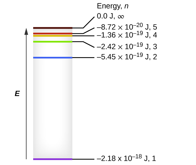
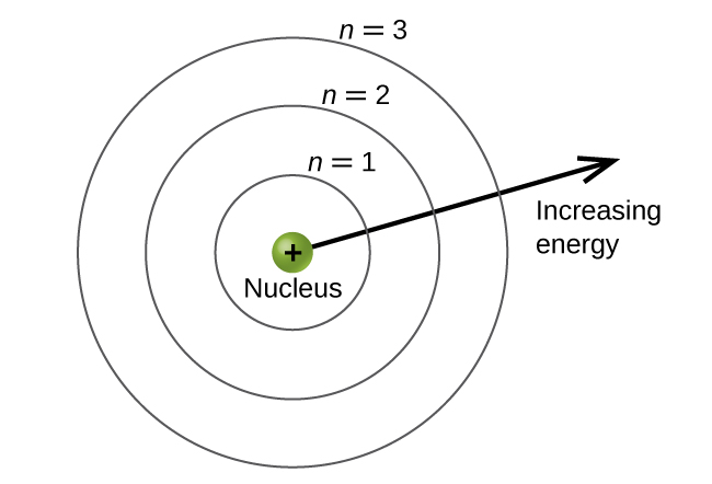
The lowest few energy levels of a hydrogen atom are shown in Figure 1. One of the fundamental laws of physics is that matter is most stable with the lowest possible energy. Thus, the electron in a hydrogen atom usually moves in the n = 1 orbit, the orbit in which it has the lowest energy, and the atom is said to be in its ground electronic state (or simply ground state). If the atom receives energy from an outside source, it is possible for the electron to move to an orbit with a higher n value and the atom is now in an excited electronic state (or simply an excited state) with a higher energy. When an electron transitions from an excited state (higher energy orbit) to a less excited state or ground state, the difference in energy is emitted as a photon. Similarly, if a photon is absorbed by an atom, the energy of the photon moves an electron from a lower energy orbit up to a more excited one.
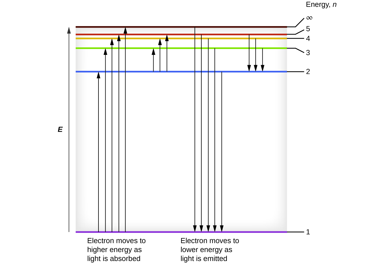
The law of conservation of energy states that we can neither create nor destroy energy. Thus, if a certain amount of external energy is required to excite an electron from one energy level to another, that same amount of energy will be liberated when the electron returns to its initial state (Figure 2). In effect, an atom can “store” energy by using it to promote an electron to a state with a higher energy and release it when the electron returns to a lower state. The energy can be released as one quantum of energy, as the electron returns to its ground state (say, from n = 5 to n = 1), or it can be released as two or more smaller quanta as the electron falls to an intermediate state, then to the ground state (say, from n = 5 to n = 4, emitting one photon, then to n = 1, emitting a second photon).
Since Bohr’s model involved only a single electron, it could also be applied to the single electron ions He+, Li2+, Be3+, etc., which differ from hydrogen only in their nuclear charges, and so one-electron systems are collectively referred to as hydrogen-like atoms. The energy expression for hydrogen-like atoms is a generalization of the hydrogen atom energy:
where Z is the nuclear charge (+1 for hydrogen, +2 for He, +3 for Li, etc.) and k has a value of 2.179 × 10⁻¹⁸ J. The sizes of the circular orbits for hydrogen-like atoms are given in terms of their radii by:
where α0 is a constant called the Bohr radius, with a value of 5.292 × 10⁻¹¹ m. The equations show us that as the electron’s energy increases (as n increases), the electron is found at greater distances from the nucleus. This is consistent with the inverse dependence on r in the Coulomb potential—as the electron moves away from the nucleus, the electrostatic attraction between it and the nucleus decreases, and it is held less tightly in the atom. Note that as n gets larger and the orbits get larger, their energies get closer to zero, and so the limits n→∞ and r→∞ imply that E = 0 corresponds to the ionization limit where the electron is completely removed from the nucleus. Thus, for hydrogen in the ground state n = 1, the ionization energy would be:
With three extremely puzzling paradoxes now solved (blackbody radiation, the photoelectric effect, and the hydrogen atom), and all involving Planck’s constant in a fundamental manner, it became clear to most physicists at that time that the classical theories that worked so well in the macroscopic world were fundamentally flawed and could not be extended down into the microscopic domain of atoms and molecules. Unfortunately, despite Bohr’s remarkable achievement in deriving a theoretical expression for the Rydberg constant, he was unable to extend his theory to the next simplest atom, He, which only has two electrons. Bohr’s model is severely flawed, since it is still based on the classical mechanics notion of precise orbits, a concept that was later found to be untenable in the microscopic domain.
Example 1
Calculating the Energy of an Electron in a Bohr Orbit
Early researchers were very excited when they were able to predict the energy of an electron at a particular distance from the nucleus in a hydrogen atom. If a spark promotes the electron in a hydrogen atom into an orbit with n = 3, what is the calculated energy, in joules, of the electron?
Solution
The energy of the electron is given by this equation:
Z = 1 for hydrogen; k = 2.179 × 10⁻¹⁸ J; and the electron is in the n = 3 orbit. Thus,
Check Your Learning
The electron is promoted even further to an orbit with n = 6. What is its new energy?
Answer:
−6.053 × 10⁻²⁰ J
Example 2
Calculating the Energy and Wavelength of Electron Transitions in a One–electron (Bohr) System
What is the energy (in joules) and the wavelength (in meters) of the line in the spectrum of hydrogen that represents the movement of an electron from Bohr orbit with n = 4 to the orbit with n = 6? In what part of the electromagnetic spectrum do we find this radiation?
Solution
In this case, n1 = 4 and n2 = 6. The difference in energy between the two states is given by this expression:
This energy difference is positive, indicating a photon enters the system (is absorbed) to excite the electron from the n = 4 orbit up to the n = 6 orbit. The wavelength of a photon with this energy is found by the expression [latex]E = \frac{hc}{\lambda}[/latex]. Rearrangement gives:
This wavelength is found in the infrared portion of the electromagnetic spectrum.
Check Your Learning
What is the energy in joules and the wavelength in meters of the photon produced when an electron falls from the n = 5 to the n = 3 level in a He+ ion (Z = 2)?
Answer:
6.198 × 10⁻¹⁹ J; 3.205 × 10⁻⁷ m
Bohr’s model of the hydrogen atom provides insight into the behavior of matter at the microscopic level, but it is does not account for electron–electron interactions in atoms with more than one electron. It does introduce several important features of all models used to describe the distribution of electrons in an atom. These features include the following:
- The energies of electrons (energy levels) in an atom are quantized, described by quantum numbers: integer numbers having only specific allowed value and used to characterize the arrangement of electrons in an atom.
- An electron’s energy increases with increasing distance from the nucleus.
- The discrete energies (lines) in the spectra of the elements result from quantized electronic energies.
Of these features, the most important is the postulate of quantized energy levels for an electron in an atom. As a consequence, the model laid the foundation for the quantum mechanical model of the atom. Bohr won a Nobel Prize in Physics for his contributions to our understanding of the structure of atoms and how that is related to line spectra emissions.
Bohr’s model explained the experimental data for the hydrogen atom and was widely accepted, but it also raised many questions. Why did electrons orbit at only fixed distances defined by a single quantum number n = 1, 2, 3, and so on, but never in between? Why did the model work so well describing hydrogen and one-electron ions, but could not correctly predict the emission spectrum for helium or any larger atoms? To answer these questions, scientists needed to completely revise the way they thought about matter.
Ch2.2 The Microscopic World
We know how matter behaves in the macroscopic world—objects that are large enough to be seen by the naked eye follow the rules of classical physics. A billiard ball moving on a table will behave like a particle: It will continue in a straight line unless it collides with another ball or the table cushion, or is acted on by some other force (such as friction). The ball has a well-defined position and velocity (or a well-defined momentum, p = mv, defined by mass m and velocity v) at any given moment. When waves interact with each other, for example, interacting waves on the surface of water, interference patterns are formed similar to those shown on Figure 3. It is clear that particles and waves are very different phenomena in the macroscopic realm.

As technological improvements allowed scientists to probe the microscopic world in greater detail, it became increasingly clear by the 1920s that very small pieces of matter follow a different set of rules from those we observe for large objects. The unquestionable separation of waves and particles was no longer the case for the microscopic world.
One of the first people to pay attention to the special behavior of the microscopic world was Louis de Broglie. He asked the question: If electromagnetic radiation can have particle-like character, can electrons and other submicroscopic particles exhibit wavelike character? In his 1925 doctoral dissertation, de Broglie extended the wave–particle duality of light that Einstein used to resolve the photoelectric-effect paradox to material particles. He predicted that a particle with mass m and velocity v (that is, with linear momentum p) should also exhibit the behavior of a wave with a wavelength value λ, given by this expression:
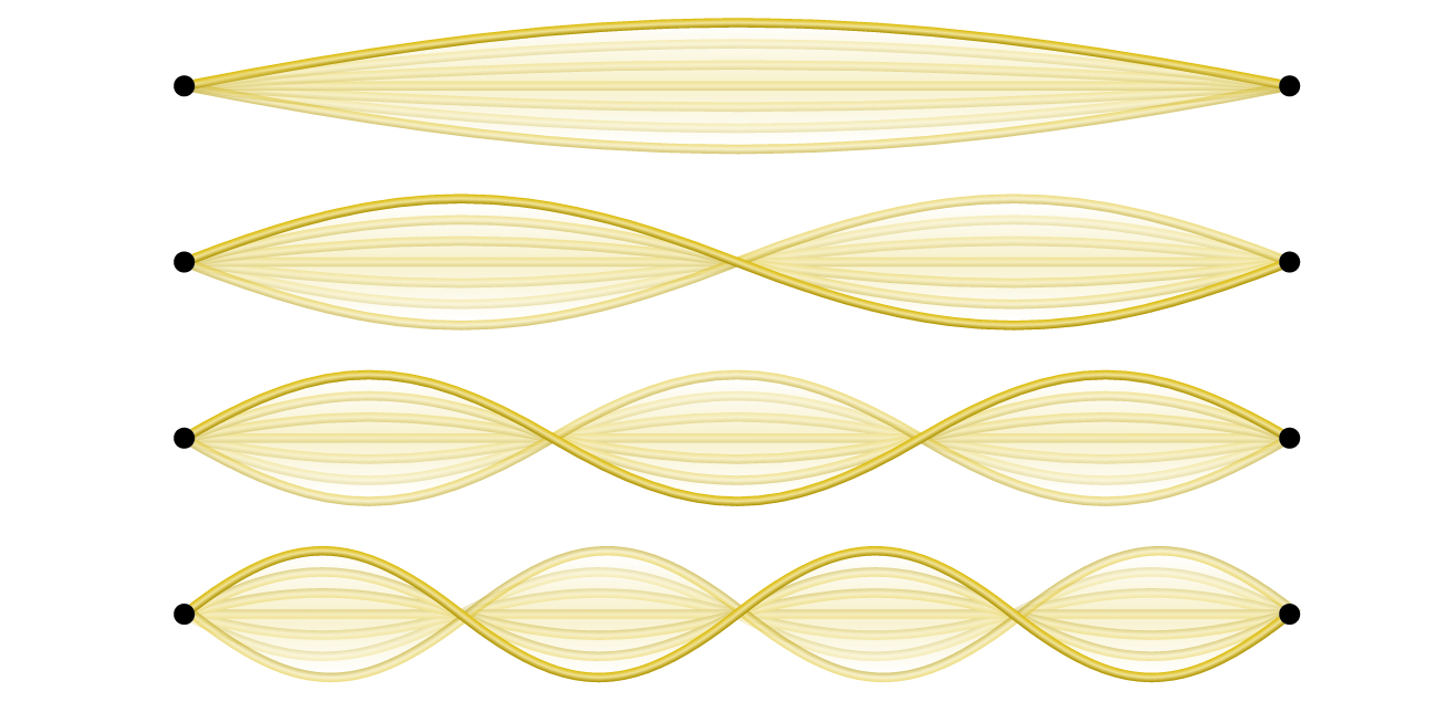
where h is the Planck’s constant. This is called the de Broglie wavelength. Unlike the other values of λ discussed in this chapter, the de Broglie wavelength is a characteristic of particles and other bodies, not electromagnetic radiation (note that this equation involves velocity [v, m/s], not frequency [ν, Hz]. Although these two symbols are identical, they mean very different things). Where Bohr had postulated the electron as being a particle orbiting the nucleus in quantized orbits, de Broglie argued that Bohr’s assumption of quantization can be explained if the electron is considered not as a particle, but rather as a circular standing wave such that only an integer number of wavelengths could fit exactly within the orbit (Figure 4).
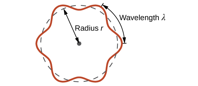
For a circular orbit of radius r, the circumference is 2πr, and so de Broglie’s condition is:
2πr = nλ, n = 1, 2, 3, …
Since the de Broglie expression relates the wavelength to the momentum and, hence, velocity, this implies:
which can be rearranged to give Bohr’s formula for the quantization of the angular momentum:
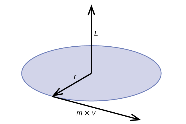
where [latex]\hbar = \frac{h}{2 \pi}[/latex]. Classical angular momentum L for a circular motion is equal to the product of the radius of the circle and the momentum of the moving particle p.
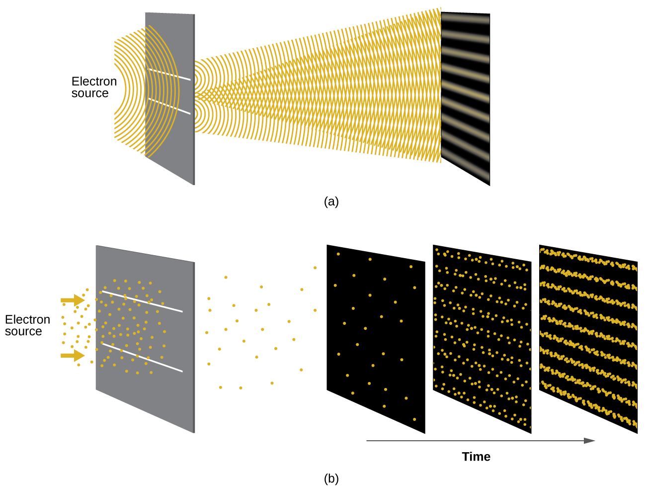
Shortly after de Broglie proposed the wave nature of matter, two scientists at Bell Laboratories, C. J. Davisson and L. H. Germer, demonstrated experimentally that electrons can exhibit wavelike behavior—they obtained an interference pattern for electrons traveling through a crystal. The regularly spaced atomic layers in a crystal served as slits in an interference experiments. Since the spacing between slits needs to be similar in size to the wavelength of the tested wave for an interference pattern to form, Davisson and Germer used a crystalline nickel target, since the spacing of the lattice was approximately the same as the de Broglie wavelengths of the electrons. Figure 6 shows an interference pattern that is strikingly similar to the interference patterns for light. The wave–particle duality of matter is also manifested in this experiment. Initially, when only a few electrons have been recorded, they show clear particle-like behavior, having arrived in localized positions that appear to be random. As more and more electrons were recorded, a clear interference pattern that is the hallmark of wavelike behavior emerge. Thus, it appears that while electrons are small localized particles, their motion does not follow the equations of motion implied by classical mechanics, but instead it is governed by some type of a wave equation that governs a probability distribution even for a single electron’s motion. Thus the wave–particle duality first observed with photons is actually a fundamental behavior intrinsic to all quantum particles.
View the Dr. Quantum – Double Slit Experiment cartoon for an easy-to-understand description of wave–particle duality and the associated experiments.
Example 3
Calculating the Wavelength of a Particle
If an electron travels at a velocity of 1.000 × 10⁷ m/s and has a mass of 9.109 × 10⁻²⁸ g, what is its wavelength?
Solution
We can use de Broglie’s equation to solve this problem, but we first must do a unit conversion of Planck’s constant, namely, 1 J = 1 kg m2/s2. Thus, we can write h = 6.626 × 10⁻³⁴ J*s = 6.626 × 10⁻³⁴ kg m2/s.
This is a small value, but it is significantly larger than the size of an electron in the classical (particle) view. This size is the same order of magnitude as the size of an atom. This means that electron’s wavelike behavior is going to be noticeable on the atom scale.
Check Your Learning
Calculate the wavelength of a softball with a mass of 100 g traveling at a velocity of 35 m/s, assuming that it can be modeled as a single particle.
Answer:
1.9 × 10⁻³⁴ m.
We never think of a thrown softball having a wavelength, since this wavelength is so small it is impossible for our senses or any known instrument to detect (strictly speaking, the wavelength of a real baseball would correspond to the wavelengths of its constituent atoms and molecules, which, while much larger than this value, would still be microscopically tiny). The de Broglie wavelength is only appreciable for matter that has a very small mass and/or a very high velocity.
Ch2.3 Standing Waves
Not all waves are traveling waves. Standing waves (also known as stationary waves) remain constrained within some region of space. As we shall see, standing waves play an important role in our understanding of the electronic structure of atoms and molecules. The simplest example of a standing wave is a one-dimensional wave associated with a vibrating string that is held fixed at its two end points. Figure 7 shows the four lowest-energy standing waves (the fundamental wave and the lowest three harmonics) for a vibrating string at a particular amplitude. Although the string’s motion lies mostly within a plane, the wave itself is considered to be one dimensional, since it lies along the length of the string. The motion of string segments in a direction perpendicular to the string length generates the waves and so the amplitude of the waves is visible as the maximum displacement of the curves seen in Figure 7. The key observation from the figure is that only those waves having an integer number, n, of half-wavelengths between the end points can form. A system with fixed end points such as this restricts the number and type of the possible waveforms. This is an example of quantization, in which only discrete values, from a more general set of continuous values of some property, are observed. Another important observation is that the harmonic waves (those waves displaying more than one-half wavelength) all have one or more points between the two end points that are not in motion. These special points are nodes. The energies of the standing waves with a given amplitude in a vibrating string increase with the number of half-wavelengths n. Since the number of nodes is n – 1, the energy can also be said to depend on the number of nodes, generally increasing as the number of nodes increases.
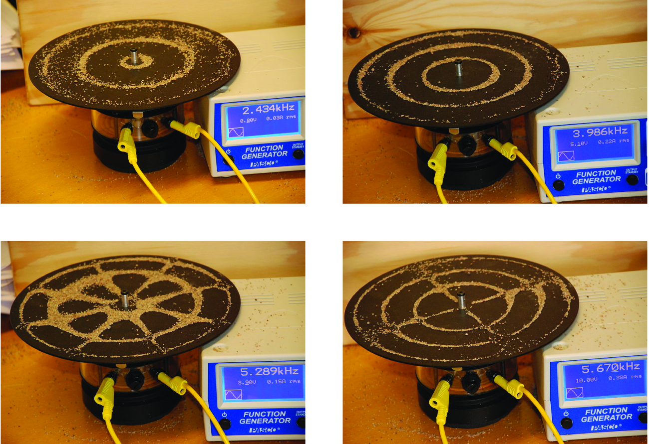
An example of two-dimensional standing waves, the vibrational patterns on a flat surface, is shown in Figure 8. Although the vibrational amplitudes cannot be seen like they could in the vibrating string, the nodes have been made visible by sprinkling the drum surface with a powder that collects on the areas of the surface that have minimal displacement. For one-dimensional standing waves, the nodes were points on the line; for two-dimensional standing waves, the nodes are lines on the surface (for three-dimensional standing waves, the nodes are two-dimensional surfaces within the three-dimensional volume). Because of the circular symmetry of the drum surface, its boundary conditions (the drum surface being tightly constrained to the circumference of the drum) result in two types of nodes: radial nodes that sweep out all angles at constant radii and, thus, are seen as circles about the center, and angular nodes that sweep out all radii at constant angles and, thus, are seen as lines passing through the center. The upper left image in Figure 8 shows two radial nodes, while the image in the lower right shows the vibrational pattern associated with three radial nodes and two angular nodes.
You can watch the formation of various radial nodes here as singer Imogen Heap projects her voice across a kettle drum.
Ch2.4 Uncertainty Principle
Werner Heisenberg considered the limits of how accurately we can measure properties of an electron or other microscopic particles. He determined that there is a fundamental limit to how accurately one can measure both a particle’s position and its momentum simultaneously. The more accurately we measure the momentum of a particle, the less accurately we can determine its position at that time, and vice versa. This is summed up in what we now call the Heisenberg uncertainty principle: It is fundamentally impossible to determine simultaneously and exactly both the momentum and the position of a particle. For a particle of mass m moving with velocity vx in the x direction (or equivalently with momentum px), the product of the uncertainty in the position, Δx, and the uncertainty in the momentum, Δpx , must be greater than or equal to [latex]\frac{\hbar}{2}[/latex]:.
For example, if we improve our measurement of an electron’s position so that the uncertainty in the position (Δx) has a value of, say, 1 pm (10–12 m, ~1% of the diameter of a hydrogen atom), then our determination of its momentum must have an uncertainty with a value of at least:
The value of ħ is small, so the uncertainty in the position or momentum of a macroscopic object like a baseball is too insignificant to observe. However, the mass of a microscopic object such as an electron is small enough that the uncertainty can be large and significant:
This means that if the uncertainty in the electron’s position is 1 pm, the uncertainty in its velocity is at least 5×10⁷ m/s. In other words, we essentially have no idea how fast it’s moving.
Heisenberg’s uncertainty principle is not just limited to uncertainties in position and momentum, it also links other dynamical variables. For example, the uncertainty in the energy and the uncertainty in the time are similarly related:
(ΔE)(Δt) ≥ [latex]\frac{\hbar}{2}[/latex]
As will be discussed later, even the vector components of angular momentum cannot all be specified exactly simultaneously.
Heisenberg’s principle imposes ultimate limits on what is measureable in science. The uncertainty principle can be shown to be a consequence of wave–particle duality, which lies at the heart of what distinguishes modern quantum theory from classical mechanics. The equations of motion obtained from classical mechanics are trajectories where, at any given instant in time, both the position and the momentum of a particle can be determined exactly. Heisenberg’s uncertainty principle implies that such a view is untenable in the microscopic domain and that there are fundamental limitations governing the motions of quantum particles. This does not mean that microscopic particles do not move in trajectories, it is just that measurements of trajectories are limited in their precision. In the realm of quantum mechanics, measurements introduce changes into the system that is being observed.
Read this article that describes a recent macroscopic demonstration of the uncertainty principle applied to microscopic objects.
Ch2.5 The Quantum–Mechanical Model of an Atom
Shortly after de Broglie published his ideas that the electron in a hydrogen atom could be better thought of as being a circular standing wave instead of a particle moving in quantized circular orbits, as Bohr had argued, Erwin Schrödinger extended de Broglie’s work by incorporating the de Broglie relation into a wave equation, deriving what is today known as the Schrödinger equation. When Schrödinger applied his equation to hydrogen-like atoms, he was able to reproduce Bohr’s expression for the energy and, thus, the Rydberg formula governing hydrogen spectra, and he did so without having to invoke Bohr’s assumptions of stationary states and quantized orbits, angular momenta, and energies; quantization in Schrödinger’s theory was a natural consequence of the underlying mathematics of the wave equation. Like de Broglie, Schrödinger initially viewed the electron in hydrogen as being a physical wave instead of a particle, but where de Broglie thought of the electron in terms of circular stationary waves, Schrödinger properly thought in terms of three-dimensional stationary waves, or wavefunctions, represented by the Greek letter psi, ψ. A few years later, Max Born proposed an interpretation of the wavefunction ψ that is still accepted today: Electrons are still particles, and so the waves represented by ψ are not physical waves but, instead, are complex probability amplitudes. The square of the magnitude of a wavefunction (|ψ|2) describes the probability of the quantum particle being present near a certain location in space. This means that wavefunctions can be used to determine the distribution of the electron’s density with respect to the nucleus in an atom. In the most general form, the Schrödinger equation can be written as:
[latex]\hat{\mathcal{H}}[/latex] is the Hamiltonian operator, a set of mathematical operations representing the total energy of the quantum particle (such as an electron in an atom), ψ is the wavefunction of this particle that can be used to find the spatial distribution of the probability of finding the particle, and E is the actual value of the total energy of the particle.
Schrödinger’s work, as well as that of Heisenberg and many other scientists following in their footsteps, is generally referred to as quantum mechanics.
You may also have heard of Schrödinger because of his famous thought experiment. This story explains the concepts of superposition and entanglement as related to a cat in a box with poison.
Ch2.6 Understanding Quantum Theory of Electrons in Atoms
The goal of this section is to understand the electron orbitals (location of electrons in atoms), their different energies, and other properties. The use of quantum theory provides the best understanding to these topics. This knowledge is a precursor to chemical bonding.
As was described previously, electrons in atoms can exist only on discrete energy levels but not between them. The energy of an electron in an atom is therefore quantized, that is, it can only be certain specific values and can jump from one energy level to another but not transition smoothly or stay between these levels.
The energy levels are labeled with an n value, where n = 1, 2, 3, etc. Generally speaking, the energy of an electron in an atom is higher for greater values of n. This number, n, is referred to as the principle quantum number. The principle quantum number defines the location of the energy level. It is essentially the same concept as the n in the Bohr atom description. Another name for the principal quantum number is the shell number. The shells of an atom can be thought of as concentric spheres radiating out from the nucleus. The electrons that belong to a specific shell are most likely to be found within the corresponding spherical area. The further we proceed from the nucleus, the higher the shell number, and higher the energy level (Figure 9). The positively charged protons in the nucleus stabilize the electronic orbitals by electrostatic attraction with the negative charges of the electrons. So the further away the electron is from the nucleus, the higher the energy it has.
This quantum mechanical model for where electrons reside in an atom can be used to look at electronic transitions, the events where an electron moves from one energy level to another. If the transition is to a higher energy level, energy is absorbed, and the energy change has a positive value. To obtain the amount of energy necessary for the transition to a higher energy level, a photon is absorbed by the atom. A transition to a lower energy level involves a release of energy, and the energy change is negative. This process is accompanied by emission of a photon by the atom. The following equation summarizes these relationships and is based on the hydrogen atom:
You have already used this equation to calculate the energy changes involved in such electronic transitions.
The principal quantum number is one of three quantum numbers used to characterize an atomic orbital. An atomic orbital, which is distinct from an orbit, is a general region in an atom within which an electron is most probable to reside. The quantum mechanical model specifies the probability of finding an electron in the three-dimensional space around the nucleus and is based on solutions of the Schrödinger equation.
Another quantum number is l, the angular momentum quantum number (or orbital quantum number). It is an integer that defines the shape of the orbital, and takes on the values, l = 0, 1, 2, …, n – 1. This means that an orbital with n = 1 can have only one value of l, l = 0, whereas n = 2 permits l = 0 and l = 1, and so on. The principal quantum number defines the general size and energy of the orbital. The l value specifies the shape of the orbital. Orbitals with the same value of l form a subshell. In addition, an electron in an orbital with a larger l value would itself have greater angular momentum. Orbitals with l = 0 are called s orbitals (or the s subshells). l = 1 corresponds to the p orbitals. The orbitals with l = 2 are called the d orbitals, followed by the f-, g-, and h-orbitals for l = 3, 4, 5.
There are certain distances from the nucleus at which the probability of finding an electron located at a particular orbital is zero. In other words, the value of the wavefunction ψ is zero at this distance for this orbital. Such a value of radius r is called a radial node. The number of radial nodes in an orbital is n – l – 1.
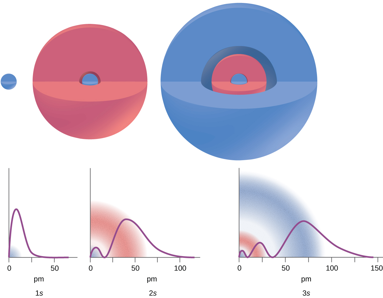
Consider the examples in Figure 10. The orbitals depicted are of the s type, thus l = 0. It can be seen from the graph of the probability densities that there are 1 – 0 – 1 = 0 places where the density is zero for a 1s (n = 1) orbital, in other words, the 1s orbital has 0 radial nodes. Similarly, a 2s orbital has 2 – 0 – 1 = 1 radial node, and a 3s orbital has 3 – 0 – 1 = 2 radial nodes.
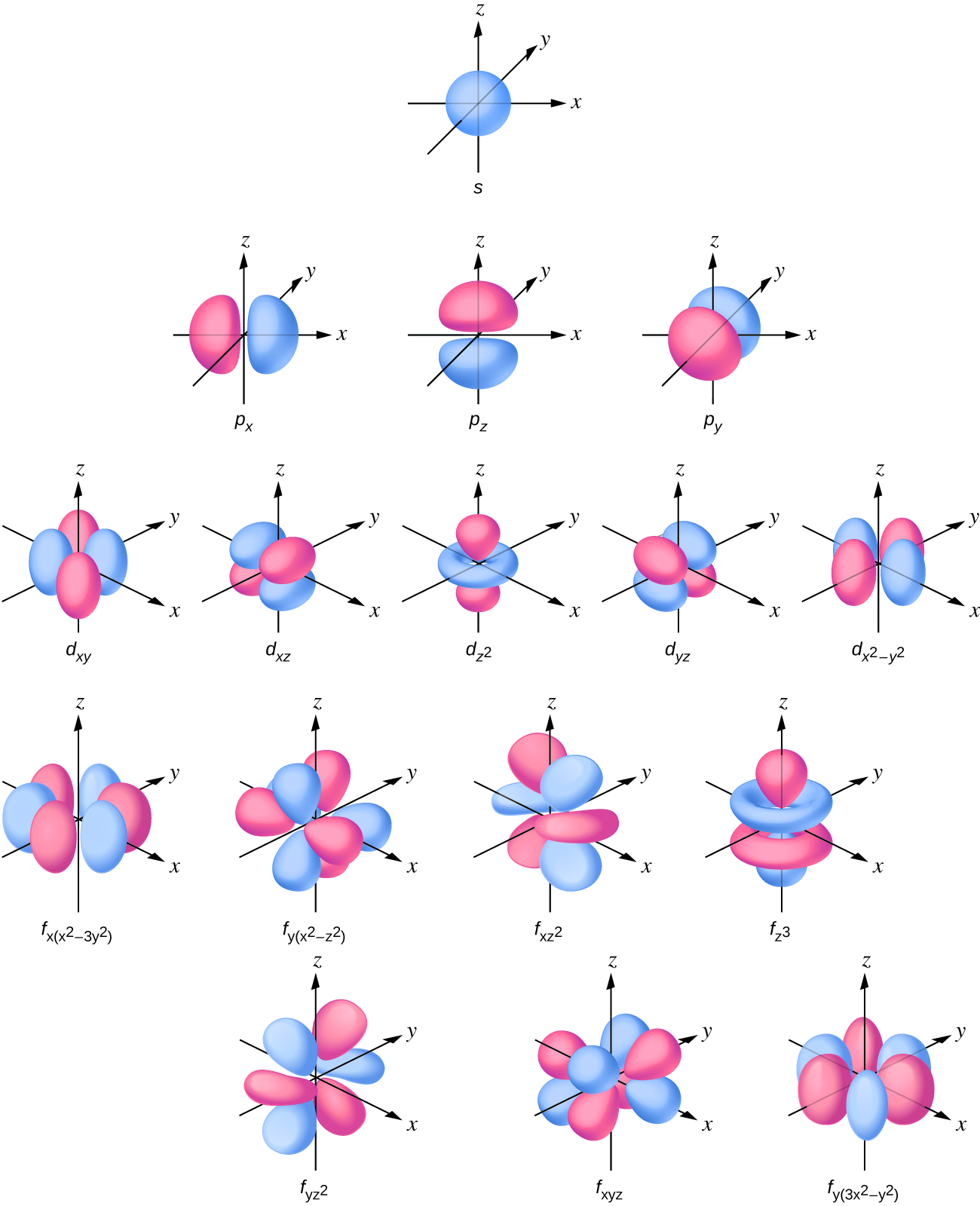
The s subshell electron density distribution is spherical, the p subshell has a dumbbell shape, and the d and f orbitals are more complex (Figure 11). These shapes represent the three-dimensional regions within which the electron is likely to be found.
If an electron has an angular momentum (l ≠ 0), then this vector can point in different directions. In addition, the z component of the angular momentum can have more than one value. This means that if a magnetic field is applied in the z direction, orbitals with different values of the z component of the angular momentum will have different energies resulting from interacting with the field. The magnetic quantum number, ml, specifies the z component of the angular momentum for a particular orbital. For example, for an s orbital, l = 0, the only value of ml is zero. For p orbitals, l = 1, ml can be equal to –1, 0, or +1. Generally speaking, ml can have the value of –l, –(l – 1), …, –1, 0, +1, …, (l – 1), l. The total number of possible orbitals with the same value of l (a subshell) is 2l + 1. Thus, there is one s-orbital for ml = 0, there are three p-orbitals for ml = –1, 0, +1, five d-orbitals for ml = -2, –1, 0, +1, +2, and so forth.
The principle quantum number defines the general size of the orbitals, the orbital quantum number determines the shape of the orbital, and the magnetic quantum number specifies orientation of the orbital in space, as can be seen in Figure 11.
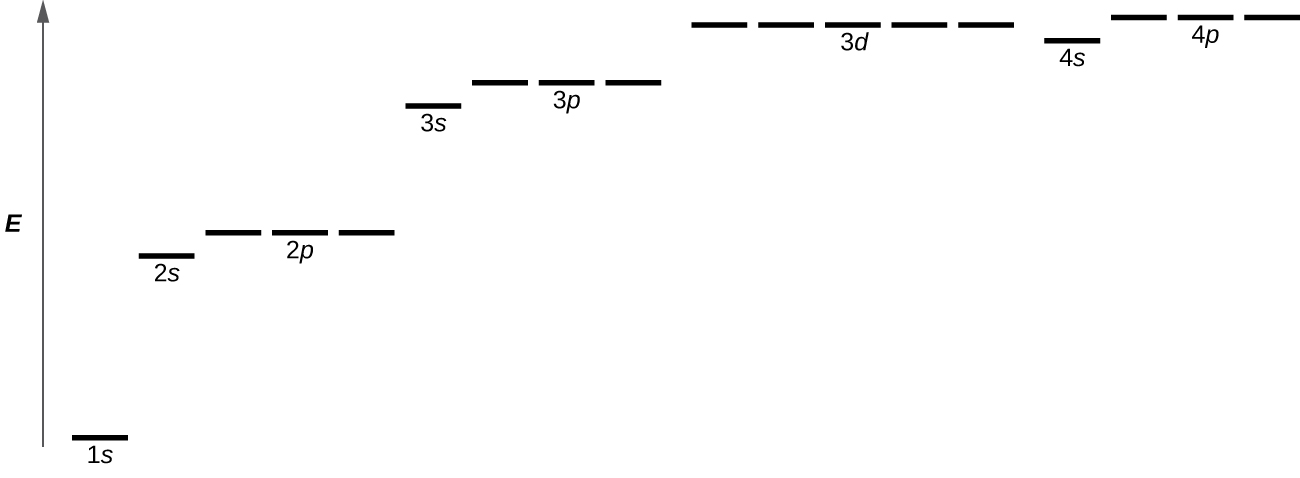
Figure 12 illustrates the energy levels for various orbitals. The number in the orbital name refers to the principle quantum number, n. The letter refers to the subshell orbital quantum number, l. Finally, there are more than one possible orbitals for l ≥ 1, each corresponding to a specific value of ml. In the case of a hydrogen atom or other one-electron system, energies of all the orbitals with the same n are the same. This is called a degeneracy, and energy levels with the same n are called degenerate energy levels. In atoms with more than one electron, some of this degeneracy is lifted by electron–electron interactions, and orbitals that belong to different subshells have different energies, as shown on Figure 12. Orbitals within the same subshell (for example the three 2p orbitals) are still degenerate and have the same energy.
While the three quantum numbers discussed above work well for describing atomic orbitals, they are insufficient to explain all observed results. It was demonstrated in the 1920s that when hydrogen line spectra are examined at extremely high resolution, some lines are actually not single peaks but, rather, pairs of closely spaced lines. This is so-called fine structure of the spectrum implies that there are additional small differences in the energies of the electrons even when they are located in the same orbital. These observations led Samuel Goudsmit and George Uhlenbeck to propose that the electrons themselves have a fourth quantum number. They called this the spin quantum number, or ms.
n, l, and ml are properties of specific atomic orbitals that also define in what part of the space an electron is most likely to be located. Orbitals are a result of solving the Schrödinger equation for electrons in atoms. The electron spin is a different kind of property. It is a completely quantum phenomenon with no analogues in the classical realm. In addition, it cannot be derived from solving the Schrödinger equation and is not related to the normal spatial coordinates (such as the Cartesian x, y, and z). Electron spin describes an intrinsic electron “rotation” or “spinning.” Each electron acts as a tiny magnet or a tiny rotating object with an angular momentum, even though this rotation cannot be observed in terms of the spatial coordinates.
The magnitude of the overall electron spin can only have one value, and an electron can only “spin” in one of two quantized states. One is termed the α state, with the z component of the spin being in the positive direction of the z axis. This corresponds to [latex]m_s = \frac{1}{2}[/latex]. The other is called the β state, with the z component of the spin being negative and [latex]m_s = -\frac{1}{2}[/latex]. Any electron, regardless of the atomic orbital it is located in, can only have one of those two values of the spin quantum number. The energies of electrons having [latex]m_s = - \frac{1}{2}[/latex] and [latex]m_s = \frac{1}{2}[/latex] are different if an external magnetic field is applied.
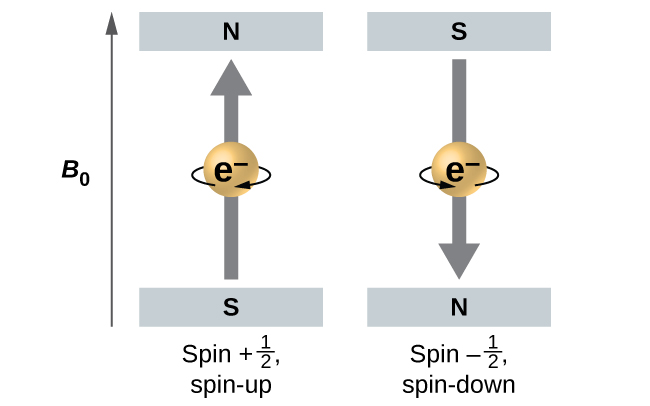
Figure 13 illustrates this phenomenon. An electron acts like a tiny magnet. A magnet has a lower energy if its magnetic moment is aligned with the external magnetic field (the left electron on Figure 13) and a higher energy for the magnetic moment is opposite to the applied field. This is why an electron with [latex]m_s = \frac{1}{2}[/latex] has a slightly lower energy in an external field in the positive z direction, and an electron with [latex]m_s = -\frac{1}{2}[/latex] has a slightly higher energy in the same field. This is true even for an electron occupying the same orbital in an atom. A spectral line corresponding to a transition for electrons from the same orbital but with different spin quantum numbers has two possible values of energy; thus, the line spectrum will show a fine structure splitting.
Ch2.7 The Pauli Exclusion Principle
An electron in an atom is completely described by four quantum numbers: n, l, ml, and ms. The first three quantum numbers define the orbital and the fourth quantum number describes the intrinsic electron property called spin. An Austrian physicist Wolfgang Pauli formulated a general principle that gives the last piece of information we need to understand the general behavior of electrons in atoms. The Pauli exclusion principle can be formulated as follows: No two electrons in the same atom can have exactly the same set of all four quantum numbers. What this means is that electrons can share the same orbital (the same set of the quantum numbers n, l, and ml), but only if their spin quantum numbers ms have different values. Since the spin quantum number can only have two values ([latex]\pm \frac{1}{2}[/latex]), no more than two electrons can occupy the same orbital (and if two electrons are located in the same orbital, they must have opposite spins). Therefore, any atomic orbital can be populated by at most two electrons.
The properties and meaning of the quantum numbers of electrons in atoms are briefly summarized in Table 1.
| Name | Symbol | Allowed values | Physical meaning |
|---|---|---|---|
| principle quantum number | n | 1, 2, 3, 4, …. | shell, the general size (and energy) of the orbital |
| angular momentum or azimuthal quantum number | l | 0 ≤ l ≤ n – 1 | subshell, the shape of the orbital |
| magnetic quantum number | ml | – l ≤ ml ≤ l | orientation of the orbital |
| spin quantum number | ms | [latex]+\frac{1}{2},\;-\frac{1}{2}[/latex] | direction of the intrinsic spin of the electron |
| Table 1. Quantum Numbers, Their Properties, and Significance | |||
Example 4
Working with Shells and Subshells
Indicate the number of subshells, the number of orbitals in each subshell, and the values of l and ml for the orbitals in the n = 4 shell of an atom.
Solution
For n = 4, l can have values of 0, 1, 2, and 3. Thus, s, p, d, and f subshells are found in the n = 4 shell of an atom. For l = 0 (the s subshell), ml can only be 0. Thus, there is only one 4s orbital. For l = 1 (p-type orbitals), m can have values of –1, 0, +1, so we find three 4p orbitals. For l = 2 (d-type orbitals), ml can have values of –2, –1, 0, +1, +2, so we have five 4d orbitals. When l = 3 (f-type orbitals), ml can have values of –3, –2, –1, 0, +1, +2, +3, and we can have seven 4f orbitals. Thus, we find a total of 16 orbitals in the n = 4 shell of an atom.
Check Your Learning
Identify the subshell in which electrons with the following quantum numbers are found: (a) n = 3, l = 1; (b) n = 5, l = 3; (c) n = 2, l = 0.
Answer:
(a) 3p (b) 5f (c) 2s
Example 5
Maximum Number of Electrons
Calculate the maximum number of electrons that can occupy a shell with (a) n = 2, (b) n = 5, and (c) n as a variable. Note you are only looking at the orbitals with the specified n value, not those at lower energies.
Solution
(a) When n = 2, there are four orbitals (a single 2s orbital, and three orbitals labeled 2p). These four orbitals can contain eight electrons.
(b) When n = 5, there are five subshells of orbitals that we need to sum:
1 5s + 3 5p + 5 5d + 7 5f + 9 5g = 25 orbitals total
Again, each orbital holds two electrons, so 50 electrons can fit in this shell.
(c) The number of orbitals in any shell n will equal n2. There can be up to two electrons in each orbital, so the maximum number of electrons will be 2 × n2
Check Your Learning
If a shell contains a maximum of 32 electrons, what is the principal quantum number, n?
Answer:
n = 4
Example 6
Working with Quantum Numbers
Complete the following table for atomic orbitals:
| Orbital | n | l | ml degeneracy | Radial nodes (no.) |
|---|---|---|---|---|
| 4f | ||||
| 4 | 1 | |||
| 7 | 7 | 3 | ||
| 5d |
Solution
The table can be completed using the following rules:
- The orbital designation is nl, where l = 0, 1, 2, 3, 4, 5, … is mapped to the letter sequence s, p, d, f, g, h, …,
- The ml degeneracy is the number of orbitals within an l subshell, 2l + 1 (there is one s orbital, three p orbitals, five d orbitals, seven f orbitals, and so forth).
- The number of radial nodes is equal to n – l – 1.
| Orbital | n | l | ml degeneracy | Radial nodes (no.) |
|---|---|---|---|---|
| 4f | 4 | 3 | 7 | 0 |
| 4p | 4 | 1 | 3 | 2 |
| 7f | 7 | 3 | 7 | 3 |
| 5d | 5 | 2 | 5 | 2 |
Check Your Learning
How many orbitals have l = 2 and n = 3?
Answer:
The five degenerate 3d orbitals
