
Unit Two
Day 19: Integrated Rate Law; Radioactive Decay
As you work through this section, if you find that you need a bit more background material to help you understand the topics at hand, you can consult “Chemistry: The Molecular Science” (5th ed. Moore and Stanitski) Chapter 11-3, 18-1 and 18-2, and/or Chapter 9.6-9.12 in the Additional Reading Materials section.
D19.1 Integrated Rate Laws
Another way to determine the rate law and rate constant from experimental data for a reaction is the integrated rate law method. An integrated rate law relates the concentration of reactant or product in a reaction mixture to the elapsed time of the reaction. Thus, an integrated rate law can be used to determine the concentration of reactant or product present after a period of time or to estimate the time required for a reaction to proceed to a certain extent. For a given rate equation, calculus can be used to derive an appropriate integrated rate law. If you are not familiar with calculus and integration, don’t worry—you can still use the integrated rate law for a reaction without deriving it yourself.
For a generic reaction:
The rate of the reaction can be expressed as:
[latex]\displaystyle{\rm{rate }} = {\rm{ }} - \frac{{\Delta {\rm{[A]}}}}{{\Delta t}}[/latex]
In calculus, the definition of a derivative is
[latex]\displaystyle\frac{{d{\rm{[A]}}}}{{dt}}{\rm{ }} = {\rm{ }}\mathop {\lim }\limits_{\Delta t \to 0} \frac{{\Delta {\rm{[A]}}}}{{\Delta t}}[/latex]
So a rate law for the reaction can be written as
Using the rules of calculus, both sides of this rate equation can be integrated to
or, assuming that the reaction starts at t = 0,
where [A]0 is the initial reactant concentration and [A]t is the reactant concentration at time t. The solution to the left side of this equation has a different mathematical form depending on the order of the reaction with respect to A (value of m). We will explore each value of m in the following sections.
D19.2 First-Order Reaction
When m = 1,
which can be alternatively expressed as:
Raising e (the base of the natural logarithm system) to the power of each side of this equation gives,
Example 1
The Integrated Rate Law for a First-Order Reaction
The rate constant for the first-order decomposition of cyclobutane, C4H8 → 2 C2H4, at 500 °C is 9.2 × 10⁻³ s−1.
How long will it take for 80.0% of a sample of C4H8 to decompose?
Solution
We use the integrated form of the rate law to answer questions regarding time:
The initial concentration of C4H8, [A]0, is not provided, but we know that 80.0% of the sample has decomposed. The concentration after 80.0% decomposition is 20.0% of [A]0, the initial concentration; that is, 0.200 × [A]0. Solve the equation for t and substitute 0.200[A]0 for [A]t:
Check Your Learning
Iodine-131 is a radioactive isotope that is used to diagnose and treat some forms of thyroid cancer. Iodine-131 decays to xenon-131 according to the equation:
The decay is first-order with a rate constant of 0.138 d−1. How many days will it take for 90% of the iodine−131 in a 0.500 M solution to decay to Xe-131?
Answer:
16.7 days
The integrated rate law for a first order reaction can also be rearranged to a standard linear equation format:
Hence, if a reaction is first order, a plot of ln[A]t vs. t must be a straight line. The slope of the plot is −k and the y-intercept is ln[A]0. If the plot is not a straight line, the reaction is not first order in A.
Example 2
Determination of Reaction Order via Graphical Method
Show that the data
| Trial | Time (h) | [H2O2] (M) |
|---|---|---|
| 1 | 0 | 1.000 |
| 2 | 6.00 | 0.500 |
| 3 | 12.00 | 0.250 |
| 4 | 18.00 | 0.125 |
| 5 | 24.00 | 0.0625 |
can be represented by a first-order rate law by graphing ln[H2O2] versus time. Determine the rate constant for decomposition of H2O2 from these data.
Solution
| Trial | Time (h) | [H2O2] (M) | ln[H2O2] |
|---|---|---|---|
| 1 | 0 | 1.000 | 0.0 |
| 2 | 6.00 | 0.500 | −0.693 |
| 3 | 12.00 | 0.250 | −1.386 |
| 4 | 18.00 | 0.125 | −2.079 |
| 5 | 24.00 | 0.0625 | −2.772 |
![A graph is shown with the label “Time ( h )” on the x-axis and “l n [ H subscript 2 O subscript 2 ]” on the y-axis. The x-axis shows markings at 6, 12, 18, and 24 hours. The vertical axis shows markings at negative 3, negative 2, negative 1, and 0. A decreasing linear trend line is drawn through five points represented at the coordinates (0, 0), (6, negative 0.693), (12, negative 1.386), (18, negative 2.079), and (24, negative 2.772).](https://wisc.pb.unizin.org/app/uploads/sites/126/2017/08/CNX_Chem_12_04_FrstOKin.jpg)
The plot of ln[H2O2] vs. time is linear, thus the reaction is first order. The rate constant for a first-order reaction is equal to the negative of the slope of the plot of ln[H2O2] versus time where:
We can use any two data points to find the slope here. (A better way is to use all pairs of data points and average the results; using only two data points ignores the rest of the data. If the data are analyzed in a spreadsheet, the slope of the line can easily be obtained from the program.) For example, the value of ln[H2O2] at t = 6.00 h is −0.693; the value when t = 12.00 h is −1.386:
Check Your Learning
Graph the following data to determine whether the reaction A → B + C is first order.
| Trial | Time (s) | [A] (M) |
|---|---|---|
| 1 | 4.0 | 0.220 |
| 2 | 8.0 | 0.144 |
| 3 | 12.0 | 0.110 |
| 4 | 16.0 | 0.088 |
| 5 | 20.0 | 0.074 |
Answer:
The plot of ln[A] vs. t is not a straight line. The equation is not first order:
![A graph, labeled above as “l n [ A ] vs. Time” is shown. The x-axis is labeled, “Time ( s )” and the y-axis is labeled, “l n [ A ].” The x-axis shows markings at 5, 10, 15, 20, and 25 hours. The y-axis shows markings at negative 3, negative 2, negative 1, and 0. A slight curve is drawn connecting five points at coordinates of approximately (4, negative 1.5), (8, negative 2), (12, negative 2.2), (16, negative 2.4), and (20, negative 2.6).](https://wisc.pb.unizin.org/app/uploads/sites/126/2017/08/CNX_Chem_12_04_CYL1_img.jpg)
D19.3 Second-Order Reaction
When m = 2,
which can be alternatively expressed as:
Example 3
The Integrated Rate Law for a Second-Order Reaction
The reaction of butadiene (C4H6) with itself produces C8H12 gas:
2 C4H6(g) → C8H12(g)
The reaction is second order with a rate constant k = 5.76 × 10⁻² M-1 min-1 under certain conditions. If the initial concentration of butadiene is 0.200 M, calculate the concentration of butadiene after 10.0 min.
Solution
Use the integrated rate law to answer questions regarding time. For a second-order reaction,
We know three variables in this equation: [A]0 = 0.200 M, k = 5.76 × 10⁻² M-1 min-1, and t = 10.0 min. Therefore, we can solve for [A]t:
[latex]\displaystyle\begin{array}{rcl} \frac{1}{[A]_t} &=& (5.76\;\times\;10^{-2}\text{M}^{-1}\text{min}^{-1})(10.0\;\text{min})\;+\;\frac{1}{0.200\;\text{M}} \\[0.5em] \frac{1}{[A]_t} &=& (5.76\;\times\;10^{-1}\text{M}^{-1})\;+\;5.00\;\text{M}^{-1} \\[0.5em] \frac{1}{[A]_t} &=& 5.58\;\text{M}^{-1} \\[0.5em] [A]_t &=& 0.179\;\text{M} \end{array}[/latex]
Therefore, after 10.0 min the concentration of butadiene is 0.179 M.
Check Your Learning
If the initial concentration of butadiene is 0.0200 M, what is the concentration after 20.0 min?
Answer:
0.0195 M
The integrated rate law for second-order reaction also has a standard linear equation format:
A plot of [latex]\dfrac{1}{[A]_t}[/latex] vs t is a straight line for a second-order reaction; the slope equals k and the y-intercept is [latex]\dfrac{1}{[A]_0}[/latex]. If the plot is not a straight line, then the reaction is not second order with respect to A.
Example 4
Determination of Reaction Order via Graphical Method
Test the data given to show whether the dimerization of C4H6 is a first- or a second-order reaction.
| Trial | Time (s) | [C4H6] (M) |
|---|---|---|
| 1 | 0 | 1.00 × 10⁻² |
| 2 | 1600 | 5.04 × 10⁻³ |
| 3 | 3200 | 3.37 × 10⁻³ |
| 4 | 4800 | 2.53 × 10⁻³ |
| 5 | 6200 | 2.08 × 10⁻³ |
Solution
In order to distinguish a first-order reaction from a second-order reaction, we plot ln[C4H6] versus t and compare it with a plot of [latex]\frac{1}{[\text{C}_4\text{H}_6]}[/latex] versus t. The values needed for these plots follow.
| Time (s) | [latex]\frac{1}{[\text{C}_4\text{H}_6]}(M^{-1})[/latex] | ln[C4H6] |
|---|---|---|
| 0 | 100 | −4.605 |
| 1600 | 198 | −5.289 |
| 3200 | 296 | −5.692 |
| 4800 | 395 | −5.978 |
| 6200 | 481 | −6.175 |
The plots are shown below. The left plot of ln[C4H6] versus t is not linear; therefore the reaction is not first order. The right plot of [latex]\frac{1}{[\text{C}_4\text{H}_6]}[/latex] versus t is linear, indicating that the reaction follows second-order kinetics.
![Two graphs are shown, each with the label “Time ( s )” on the x-axis. The graph on the left is labeled, “l n [ C subscript 4 H subscript 6 ],” on the y-axis. The graph on the right is labeled “1 divided by [ C subscript 4 H subscript 6 ],” on the y-axis. The x-axes for both graphs show markings at 3000 and 6000. The y-axis for the graph on the left shows markings at negative 6, negative 5, and negative 4. A decreasing slightly concave up curve is drawn through five points at coordinates that are (0, negative 4.605), (1600, negative 5.289), (3200, negative 5.692), (4800, negative 5.978), and (6200, negative 6.175). The y-axis for the graph on the right shows markings at 100, 300, and 500. An approximately linear increasing curve is drawn through five points at coordinates that are (0, 100), (1600, 198), (3200, 296), and (4800, 395), and (6200, 481).](https://wisc.pb.unizin.org/app/uploads/sites/126/2017/08/CNX_Chem_12_04_2OrdKin.jpg)
Check Your Learning
Do these data fit a second-order rate law?
| Trial | Time (s) | [A] (M) |
|---|---|---|
| 1 | 5 | 0.952 |
| 2 | 10 | 0.625 |
| 3 | 15 | 0.465 |
| 4 | 20 | 0.370 |
| 5 | 25 | 0.308 |
| 6 | 35 | 0.230 |
Answer:
Yes. The plot of [latex]\frac{1}{[A]}[/latex] vs. t is linear:
![A graph, with the title “1 divided by [ A ] vs. Time” is shown, with the label, “Time ( s ),” on the x-axis. The label “1 divided by [ A ]” appears left of the y-axis. The x-axis shows markings beginning at zero and continuing at intervals of 10 up to and including 40. The y-axis on the left shows markings beginning at 0 and increasing by intervals of 1 up to and including 5. A line with an increasing trend is drawn through six points at approximately (4, 1), (10, 1.5), (15, 2.2), (20, 2.8), (26, 3.4), and (36, 4.4).](https://wisc.pb.unizin.org/app/uploads/sites/126/2017/08/CNX_Chem_12_04_CYL2_img.jpg)
D19.4 Zeroth-Order Reaction
When m = 0,
A zeroth-order reaction exhibits a constant reaction rate, regardless of the concentration of reactant A:
The integrated rate law for a zeroth-order reaction also has has a standard linear equation format:
A plot of [A]t vs t for a zeroth-order reaction is a straight line with a slope of −k and an intercept of [A]0.
Figure 1 shows a plot of [NH3] vs t for the decomposition of ammonia on a hot tungsten (W) wire and on hot quartz (SiO2). The decomposition on hot tungsten is zeroth-order; the plot is a straight line. From the slope, we can determine the rate constant:
The decomposition on hot quartz is not zeroth order (analysis of the data shows that it is first order).
![A graph is shown with the label, “Time ( s ),” on the x-axis and, “[ N H subscript 3 ] M,” on the y-axis. The x-axis shows a single value of 1000 marked near the right end of the axis. The vertical axis shows markings at 1.0 times 10 superscript negative 3, 2.0 times 10 superscript negative 3, and 3.0 times 10 superscript negative 3. A decreasing linear trend line is drawn through six points at the approximate coordinates: (0, 2.8 times 10 superscript negative 3), (200, 2.6 times 10 superscript negative 3), (400, 2.3 times 10 superscript negative 3), (600, 2.0 times 10 superscript negative 3), (800, 1.8 times 10 superscript negative 3), and (1000, 1.6 times 10 superscript negative 3). This line is labeled “Decomposition on W.” A decreasing slightly concave up curve is similarly drawn through eight points at the approximate coordinates: (0, 2.8 times 10 superscript negative 3), (100, 2.5 times 10 superscript negative 3), (200, 2.1 times 10 superscript negative 3), (300, 1.9 times 10 superscript negative 3), (400, 1.6 times 10 superscript negative 3), (500, 1.4 times 10 superscript negative 3), and (750, 1.1 times 10 superscript negative 3), ending at about (1000, 0.7 times 10 superscript negative 3). This curve is labeled “Decomposition on S i O subscript 2.”](https://wisc.pb.unizin.org/app/uploads/sites/126/2017/08/CNX_Chem_12_04_AmDecomK.jpg)
D19.5 Flooding: Pseudo-Order Methods
The integrated rate laws are quite useful when determining the reaction order and rate constants using all the data from a single experimental trial run. However, thus far we’ve only considered example reactions involving one reactant, whereas many reactions involve two or more reactants. How can we use integrated rate laws to find the reaction order and rate constants for those reactions?
Let’s consider the reaction
where
Flooding refers to running a reaction that involves two or more reactants with a large excess of all but one reactant. For example, run the reaction above with a large excess of reactant B so that A is the limiting reactant by a significant amount. If [B]0 >> [A]0, reactant B concentration effectively remains constant during the reaction. (If [B]0 = 0.100 M and [A]0 = 0.00100, then at a time t when all the A has reacted, [B]t = (0.100-0.001) M = 0.099 M, which is almost no change in the B concentration.) Under this condition of [B]t ≈ [B]0 = constant, the rate law becomes
where kobs, the rate constant we observe during the flooded experiment, is kobs = k[B]0n. This rate equation allows us to use the integrated rate laws we’ve just discussed to determine the reaction order with respect to reactant A and to determine kobs.
Here is an example: Flood the reaction mixture with a large excess of reactant B ([latex][B]_{0_1}[/latex]) and measure [A]t as the reaction progresses. Then plot ln[A]t vs t. If the graph is a straight line, then the reaction is first order with respect to A. (In this case, we call the flooded reaction a pseudo-first-order reaction.) The negative of the slope of the graph is [latex]k_{obs_1}[/latex].
Then run another trial with a different, large excess concentration of B, [latex][B]_{0_2}[/latex]. The plot of ln[A]t vs t has a different slope corresponding to [latex]-k_{obs_2}[/latex]. The ratio of the two kobs
allows us to determine n, the reaction order with respect to reactant B, because all other variables in the equation are known or have been experimentally determined. Finally, the actual rate constant for the reaction, k, can be determined from the relationship kobs = k[B]0n.
D19.6 Radioactive Decay
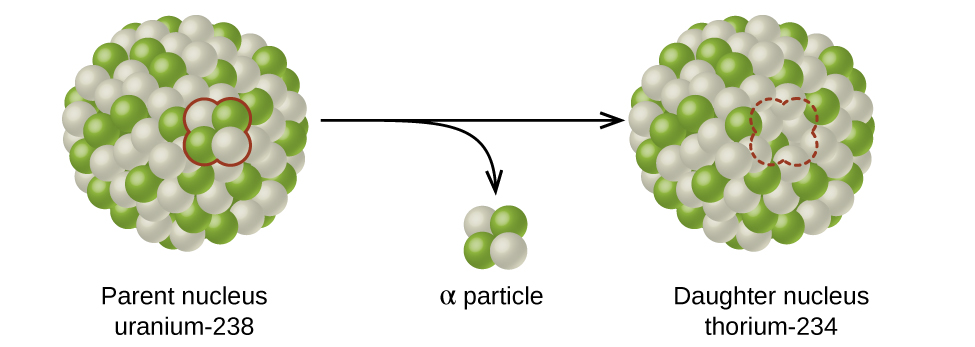
Determining the rate law and rate constant has many real world applications. An important one of these is the rate of radioactive decay, the spontaneous change of an unstable nuclide into a different nuclide. The unstable nuclide is called the parent nuclide; the nuclide that results from the decay is known as the daughter nuclide (Figure 2). The daughter nuclide may be stable, or it may decay itself.
The atomic representations used when discussing radioactive decay reactions have two numbers written to the left of the atomic symbol, for example, [latex]^{238}_{\;92}\text{U}[/latex] and its isotope [latex]^{235}_{\;92}\text{U}[/latex]. The subscript denotes the atomic number of the element (number of protons), and the superscript denotes the mass number of the isotope (number of protons + number of neutrons). Both subscript and superscript are necessary for balancing nuclear equations.
Exercise 1: Atoms and Isotopes
A typical periodic table entry for chlorine is 
(For these questions, accepted answers include numbers and/or “it depends on the isotope”.)
D19.7 Types of Radioactive Decay
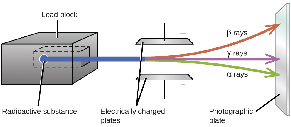
Ernest Rutherford’s experiments involving the interaction of radiation with a magnetic or electric field (Figure 3) helped him determine that one type of radiation consisted of positively charged and relatively massive α particles, which are high-energy helium nuclei ([latex]_2^4\text{He}[/latex], or [latex]_2^4{\alpha}[/latex]); a second type consisted of negatively charged and much lighter β particles, which are high-energy electrons ([latex]_{-1}^{\;\;0}{\beta}[/latex], or [latex]_{-1}^{\;\;0}\text{e}[/latex]); and a third was uncharged electromagnetic waves, γ rays, which are are photons of very high energy. Note that for beta particles, which do not contain any protons, the subscript denotes the charge of the particle.
Alpha (α) decay is the emission of an α particle from the nucleus. For example, polonium-210 undergoes α decay:
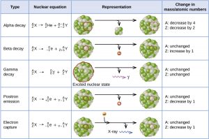
Alpha decay occurs primarily in heavy nuclei (A > 200, Z > 83). The loss of an α particle gives a daughter nuclide with a mass number four units smaller and an atomic number two units smaller than those of the parent nuclide. Note that the sum of protons (subscripts) on the product side is equal to that on the reactant side. Theame is true for the mass number (superscripts). This nuclear reaction is balanced.
Beta (β) decay is the emission of an electron from a nucleus. Iodine-131 is an example of a nuclide that undergoes β decay:
Beta decay involves the conversion of a neutron into a proton and a β particle. The β particle emitted is from the atomic nucleus and is not one of the electrons surrounding the nucleus. Emission of a β particle does not change the mass number of the nuclide but does increase the number of its protons and decrease the number of its neutrons.
Gamma (γ) decay is the emission of a γ-ray photon from a nucleus. The energies of γ rays are quite high, in the range of hundreds of thousands to tens of millions of kJ/mol, so γ rays can easily break chemical bonds if they are absorbed by matter. (In comparison, x-rays have energies roughly 10 times smaller than γ rays.) Cobalt-60 is an example nuclide that decays via β emission as well as γ emission:
The asterisk (*) denotes that Nickel-60 is in an excited state. It decays to its ground state with the emission of another γ photon:
There is no change in mass number or atomic number during γ emission unless it is accompanied by one of the other modes of decay.
Positron (β+) decay is the emission of a positron, or antielectron, from a nucleus. In the process, a proton is converted into a neutron. Oxygen-15 is an example of a nuclide that undergoes positron emission:
Electron capture occurs when one of the inner electrons in an atom is captured by the atom’s nucleus and transforms a proton into a neutron. For example, potassium-40 undergoes electron capture:
Electron capture has the same effect on the nucleus as does positron emission. Whether electron capture or positron emission occurs is difficult to predict. The choice is primarily due to kinetic factors.
Figure 4 summarizes these types of decay.
Exercise 2: Radioactive Decay
Exercise 3: Radioactive Decay and Transmutation of Elements
Podia Question
In Example 2, earlier in today’s work, data are given for the decomposition of hydrogen peroxide. Hydrogen peroxide decomposes to form oxygen and water. Write a balanced chemical equation for decomposition of hydrogen peroxide. How is the equation you wrote for hydrogen peroxide different from the chemical equation A → products that was used to derive the integrated rate law in Section D19.1?
Now define the rate of reaction for decomposition of hydrogen peroxide using the method given in Section D18.2 (the previous pre-class work) and derive the integrated first-order rate law, following the derivation in Sections D19.1 and D19.2. Use your mathematical work to show that the rate constant calculated in Example 2 for the first-order decomposition of hydrogen peroxide is twice as big as it should be.
Two days before the next whole-class session, this Podia question will become live on Podia, where you can submit your answer.
