
Unit Three
Day 29: Chemical Equilibrium
As you work through this section, if you find that you need a bit more background material to help you understand the topics at hand, you can consult “Chemistry: The Molecular Science” (5th ed. Moore and Stanitski) Chapter 12-3 through 12-5, and/or Chapter 13.4-13.9 in the Additional Reading Materials section.
D29.1 Equilibrium Constant and Partial Pressure
Reactions in which all reactants and products are in the gas phase are another class of homogeneous equilibria. In these cases, the partial pressure of each gas can be used instead of its concentration in the equilibrium constant equation because the partial pressure of a gas is directly proportional to its molar concentration (c) at constant temperature. The molar concentration is the amount of a substance (moles) per unit volume (liters): c = n/V. This proportionality of pressure and concentation can be derived from the ideal gas equation:
In a mixture of gases the partial pressure of each gas is proportional to its concentration. Using the partial pressures of the gases, we can write the equilibrium constant for this example reaction
by following the same guidelines for deriving concentration-based expressions:
where Kp designates an equilibrium constant derived using partial pressures of reactants and products.
The two equilibrium constants, Kc and Kp, are directly related to each other. For example, for the generic gas-phase reaction
where Δn is the difference between the sum of the coefficients of the gaseous products and reactants in the reaction (i.e., the change in amount of gas between the reactants and the products).
Note that the gas constant, R, can be expressed in different units. Use the R value and associated units that match the partial pressure units used in the Kp expression.
For heterogeneous equilibria that involve gases, equilibrium constants can also be expressed using partial pressures instead of concentrations. Two examples are:
Example 1
Calculation of KP
1. Write the equations for the conversion of Kc to KP for each of these reactions:
(a) [latex]\text{C}_2\text{H}_6(g)\;{\rightleftharpoons}\;\text{C}_2\text{H}_4(g)\;+\;\text{H}_2(g)[/latex]
(b) [latex]\text{CO}(g)\;+\;\text{H}_2\text{O}(g)\;{\rightleftharpoons}\;\text{CO}_2(g)\;+\;\text{H}_2(g)[/latex]
(c) [latex]\text{N}_2(g)\;+\;3\;\text{H}_2(g)\;{\rightleftharpoons}\;2\;\text{NH}_3(g)[/latex]
2. Kc is equal to 0.28 M−2 for this reaction at 900 °C:
Calculate KP at this temperature.
Solution
1. (a) Δn = (2) − (1) = 1
KP = Kc (RT)Δn = Kc (RT)1 = Kc (RT)
(b) Δn = (2) − (2) = 0
KP = Kc (RT)Δn = Kc (RT)0 = Kc
(c) Δn = (2) − (1 + 3) = −2
KP = Kc (RT)Δn = Kc (RT)−2 = [latex]\dfrac{K_c}{(RT)^2}[/latex]
2. For this reaction, Δn = −2. Thus,
KP = Kc (RT)Δn = [0.28 (mol/L)−2][(0.0821 [latex]\frac{\text{L}{\cdot}\text{atm}}{\text{mol}{\cdot}\text{K}}[/latex])((900 + 273) K)]−2 = 3.0 × 10⁻⁵ atm−2
To calculate the equilibrium constant in units of bar−2, we could have used the gas constant 8.314 × 10⁻² [latex]\frac{\text{L}{\cdot}\text{bar}}{\text{mol}{\cdot}\text{K}}[/latex]
Check Your Learning
1. Write the equations for the conversion of Kc to KP for each of these gas-phase reactions:
(a) [latex]2\;\text{SO}_2(g)\;+\;\text{O}_2(g)\;{\rightleftharpoons}\;2\;\text{SO}_3(g)[/latex]
(b) [latex]\text{N}_2\text{O}_4(g)\;{\rightleftharpoons}\;2\;\text{NO}_2(g)[/latex]
(c) [latex]\text{C}_3\text{H}_8(g)\;+\;5\;\text{O}_2(g)\;{\rightleftharpoons}\;3\;\text{CO}_2(g)\;+\;4\;\text{H}_2\text{O}(g)[/latex]
2. At 227 °C, this reaction has Kc = 0.0952 M2:
Calculate the value of Kp at this temperature.
Answer:
(a) KP = Kc (RT)−1; (b) KP = Kc (RT); (c) KP = Kc (RT); (d) 160 atm2 or 1.6 × 10² atm2
D29.2 Calculations Involving Equilibrium Constant
One way to determine the value for an equilibrium constant is to measure the concentrations (or partial pressures) of all reactants and all products at equilibrium and substitute into the equilibrium constant expression.
Exercise 1: Calculating an Equilibrium Constant
Calculate the equilibrium constant Kc for the decomposition of PCl5 at 250 °C.
At equilibrium, [PCl5] = 4.2 × 10⁻⁵ M, [PCl3] = 1.3 × 10⁻² M, [Cl2] = 3.9 × 10⁻³ M
Example 2
Evaluating an equilibrium constant
Gaseous nitrogen dioxide forms dinitrogen tetraoxide according to this equation:
In a 1.0-L flask at 25 °C, the concentrations at equilibrium are [NO2] = 0.016 M and [N2O4] = 0.042 M. Calculate the equilibrium constant for the reaction.
Solution
At equilibrium
[latex]K_\text{c} = \dfrac{[\text{N}_2\text{O}_4]}{[\text{NO}_2]^{2}} = \dfrac{0.042\;\text{M}}{(0.016\;\text{M})^2} = 1.6\;\times\;10^{2}\; \text{M}^{-1}[/latex]
Note that dimensional analysis gives the unit for this Kc as M−1.
Check Your Learning
For the reaction [latex]2\;\text{SO}_2(g)\;+\;\text{O}_2(g)\;{\rightleftharpoons}\;2\;\text{SO}_3(g)[/latex], the concentrations at equilibrium are [SO2] = 0.90 M, [O2] = 0.35 M, and [SO3] = 1.1 M. Calculate the equilibrium constant, Kc.
Answer:
Kc = 4.3 M−1
A known equilibrium constant can be used to calculate an unknown equilibrium concentration, provided the equilibrium concentrations of all other reactants and products are known.
Example 3
Calculation of a Missing Equilibrium Concentration
Nitrogen oxides are air pollutants produced by the reaction of nitrogen and oxygen at high temperatures. At 2000 °C, the value of the equilibrium constant for the reaction, [latex]\text{N}_2(g)\;+\;\text{O}_2(g)\;{\rightleftharpoons}\;2\;\text{NO}(g)[/latex], is Kc = 4.1 × 10⁻⁴. Find the concentration of NO(g) in an equilibrium mixture with air at 1 atm pressure at this temperature. In air, [N2] = 0.036 mol/L and [O2] 0.0089 mol/L.
Solution
We are given all of the equilibrium concentrations except that of NO. Thus, we can solve for the missing equilibrium concentration by rearranging the equation for the equilibrium constant.
Thus [NO] = 3.6 × 10⁻⁴ mol/L at equilibrium under these conditions.
Check Your Learning
The equilibrium constant for the reaction of nitrogen and hydrogen to produce ammonia at a certain temperature is 6.00 × 10⁻². Calculate the equilibrium concentration of ammonia if the equilibrium concentrations of nitrogen and hydrogen are 4.26 M and 2.09 M, respectively.
Answer:
1.53 mol/L
The magnitude of an equilibrium constant is a measure of the yield of a reaction when it reaches equilibrium. A very large value for Kc (Kc >> 1) indicates that product concentrations are much larger than reactant concentrations when equilibrium has been achieved: nearly all reactants have been converted into products. Such a reaction is product-favored. If Kc is large enough, the reaction has gone essentially to completion when it reaches equilibrium. A very small value of Kc, (Kc << 1) indicates that equilibrium is achieved when only a small proportion of the reactants have been converted into products. Such a reaction is reactant-favored. If Kc is small enough, essentially no reaction has occurred when equilibrium is reached. When Kc ≈ 1, both reactant and product concentrations are significant and it is necessary to use the equilibrium constant to calculate equilibrium concentrations. (The symbol ≈ means “approximately equal to”.)
Exercise 2: Identifying Reactant-Favored and Product-Favored Processes
D29.3 ICE Table
For a reaction that reaches equilibrium, the initial concentrations of reactants are usually known. If the equilibrium concentration of one species can be measured, an ICE table (for Initial, Change, and Equilibrium) is a good methodology for calculating an equilibrium constant. An ICE table is generated beginning with the balanced reaction equation. Below the equation the initial concentrations of the reactants and products are listed: these initial concentrations can usually be calculated from experimental data based on the assumption that no reaction has yet taken place. The next row of data is the change that occurs as the system shifts toward equilibrium: the changes in concentration are derived from the stoichiometry of the reaction. The last row is the sum of the first two rows: the concentrations once equilibrium has been reached.
For example, consider this reaction:
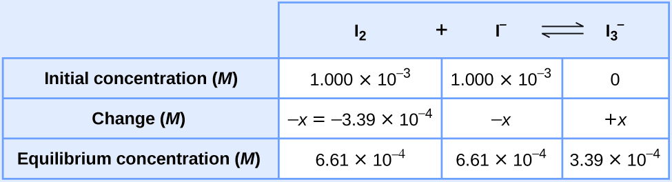
If a solution starting with [I2] = [I−] = 1.000 × 10⁻³ M and no triiodide ions, and gives an equilibrium concentration of I2 of 6.61 × 10⁻⁴ M, we can use the ICE table to determine the equilibrium constant for the reaction.
First, we set up an ICE table using −x as the change in concentration of I2. (Because the concentration of a reactant like I2 decreases as reaction occurs, the change is given a negative sign.)
![This table has two main columns and four rows. The first row for the first column does not have a heading and then has the following in the first column: Initial concentration ( M ), Change ( M ), Equilibrium concentration ( M ). The second column has the header, “I subscript 2 plus sign I superscript negative sign equilibrium arrow I subscript 3 superscript negative sign.” Under the second column is a subgroup of three rows and three columns. The first column has the following: 1.000 times 10 to the negative third power, negative x, [ I subscript 2 ] subscript i minus x. The second column has the following: 1.000 times 10 to the negative third power, negative x, [ I superscript negative sign ] subscript i minus x. The third column has the following: 0, positive x, [ I superscript negative sign ] subscript i plus x.](https://wisc.pb.unizin.org/app/uploads/sites/126/2017/08/CNX_Chem_13_04_ICETable1_img.jpg)
In the “Change” row, the mathematical sign indicates the direction of change: the sign is positive when the concentration increases as the reaction approaches equilibrium, and negative when the concentration decreases. The number x is multiplied by depends on stoichiometry: in this case all coefficients in the chemical equation are 1, so each x in the second row has a multiplier of 1 or −1.
Because the equilibrium concentration of I2 is given as 6.61 × 10⁻⁴ M, we can use the first equation in the last row to solve for x:
Now we can fill in the ICE table with the concentrations at equilibrium.
From the equilibrium concentrations in the last row, we can calculate the equilibrium constant.
Example 4
Determining Relative Changes in Concentration
Complete the changes in concentrations for each reaction.
(a) [latex]\begin{array}{lcccc} \text{C}_2\text{H}_2(g) & + & \;2\text{Br}_2(g) & {\rightleftharpoons} & \text{C}_2\text{H}_2\text{Br}_4(g) \\[0.5em] \;\;\; -x & & \rule[0ex]{2.5em}{0.1ex} & & \rule[0ex]{2.5em}{0.1ex} \end{array}[/latex]
(b) [latex]\begin{array}{lcccc} \text{I}_2(aq) & + & \text{I}^{-}(aq) & {\rightleftharpoons} & \text{I}_3^{\;\;-}(aq) \\[0.5em] \rule[0ex]{2.5em}{0.1ex} & & \rule[0ex]{2.5em}{0.1ex} & & x \end{array}[/latex]
(c) [latex]\begin{array}{lcccccc} \text{C}_3\text{H}_8(g) & + & 5\;\text{O}_2(g) & {\rightleftharpoons} & 3\;\text{CO}_2(g) & + & 4\;\text{H}_2\text{O}(g) \\[0.5em] \;\;\; -x & & \rule[0ex]{2.5em}{0.1ex} & & \rule[0ex]{2.5em}{0.1ex} & & \rule[0ex]{2.5em}{0.1ex} \end{array}[/latex]
Solution
(a) [latex]\begin{array}{lcccc} \text{C}_2\text{H}_2(g) & + & 2\text{Br}_2(g) & {\rightleftharpoons} & \text{C}_2\text{H}_2\text{Br}_4(g) \\[0.5em] \;\;\; -x & & -2x & & x \end{array}[/latex]
(b) [latex]\begin{array}{lcccc} \text{I}_2(aq) & + & \text{I}^{-}(aq) & {\rightleftharpoons} & \text{I}_3^{\;\;-}(aq) \\[0.5em] \;\; -x & & -x & & x \end{array}[/latex]
(c) [latex]\begin{array}{lcccccc} \text{C}_3\text{H}_8(g) & + & 5\text{O}_2(g) & {\rightleftharpoons} & 3\text{CO}_2(g) & + & 4\text{H}_2\text{O}(g) \\[0.5em] \;\;\; -x & & -5x & & 3x & & 4x \end{array}[/latex]
Check Your Learning
Complete the changes in concentrations for each of the following reactions:
(a) [latex]\begin{array}{lcccc} 2\;\text{SO}_2(g) & + & \text{O}_2(g) & {\rightleftharpoons} & 2\;\text{SO}_3(g) \\[0.5em] \rule[0ex]{2.5em}{0.1ex} & & -x & & \rule[0ex]{2.5em}{0.1ex} \end{array}[/latex]
(b) [latex]\begin{array}{lcc} \text{C}_4\text{H}_8(g) & {\rightleftharpoons} & 2\;\text{C}_2\text{H}_4(g) \\[0.5em] \rule[0ex]{2.5em}{0.1ex} & & 2x \end{array}[/latex]
(c) [latex]\begin{array}{lcccccc} 4\;\text{NH}_3(g) & + & 7\;\text{H}_2\text{O}(g) & {\rightleftharpoons} & 4\;\text{NO}_2(g) & + & 6\;\text{H}_2\text{O}(g) \\[0.5em] \rule[0ex]{2.5em}{0.1ex} & & \rule[0ex]{2.5em}{0.1ex} & & \rule[0ex]{2.5em}{0.1ex} & & \rule[0ex]{2.5em}{0.1ex} \end{array}[/latex]
Answer:
(a) −2x, −x, 2x; (b) −x, 2x; (c) −4x, −7x, 4x, 6x or 4x, 7x, −4x, −6x
If we know the equilibrium constant for a reaction and a set of concentrations of reactants and products that are not at equilibrium, we can calculate the changes in concentrations as the system comes to equilibrium as well as the new concentrations at equilibrium. The typical procedure can be summarized in four steps.
- Balance the chemical reaction equation and determine the direction the reaction proceeds to come to equilibrium.
- Determine the relative changes needed to reach equilibrium. Represent the smallest change with the symbol x, express the other changes in terms of x, and then write the equilibrium concentrations in terms of these changes.
- Substitute the equilibrium concentrations into the expression for the equilibrium constant, solve for x, and check any assumptions used to find x. Then calculate the equilibrium concentrations.
- Check the arithmetic by substituting the calculated equilibrium concentrations into the equilibrium constant expression and determining whether they give the equilibrium constant
Example 5
Calculation of Concentration Changes as a Reaction Goes to Equilibrium
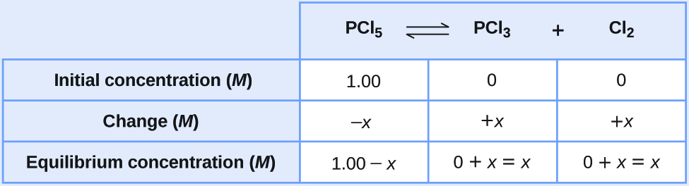
Under certain conditions, the equilibrium constant for the decomposition of PCl5(g) into PCl3(g) and Cl2(g) is Kc = 0.0211 M. Calculate the equilibrium concentrations of PCl5, PCl3, and Cl2 if the initial concentrations were [PCl5] = 1.00 M , [PCl3] = [Cl2] = 0.
Solution
Use the stepwise process described earlier.
- Balance the chemical equation and determine the direction the reaction proceeds.
The balanced equation for the decomposition of PCl5 is
[latex]\text{PCl}_5(g)\;{\rightleftharpoons}\;\text{PCl}_3(g)\;+\;\text{Cl}_2(g)[/latex]Because there are no products initially, the reaction proceeds to the right.
- Determine the relative changes needed to reach equilibrium, then write the equilibrium concentrations in terms of these changes.
Represent the increase in concentration of PCl3 by the symbol x. The other changes may be written in terms of x by considering the coefficients in the chemical equation.
[latex]\begin{array}{lcccc} \text{PCl}_5(g) & {\rightleftharpoons} & \text{PCl}_3(g) & + & \text{Cl}_2(g) \\[0.5em] -x & & x & & x \end{array}[/latex]The changes in concentration and the expressions for the equilibrium concentrations are:
- Solve for x and the equilibrium concentrations.
Substituting the equilibrium concentrations into the equilibrium constant equation gives
[latex]K_c = \dfrac{[\text{PCl}_3][\text{Cl}_2]}{[\text{PCl}_5]} = \dfrac{(x\;\text{M})(x\;\text{M})}{(1.00\;-\;x)\;\text{M}} = 0.0211\;\text{M}[/latex]This equation contains only one variable, x, the change in concentration. We can write the equation as a quadratic equation:
[latex]0.0211 = \dfrac{(x)(x)}{(1.00\;-\;x)}[/latex][latex]0.0211(1.00\;-\;x) = x^2[/latex][latex]x^2\;+\;0.0211x\;-\;0.0211 = 0[/latex]and solve for x using the quadratic formula. For an equation of the form ax2 + bx + c = 0,
[latex]x = \dfrac{-b\;{\pm}\;\sqrt{b^2\;-\;4ac}}{2a}[/latex]Here, a = 1, b = 0.0211, and c = −0.0211, which yields:
[latex]\begin{array}{rcl} x & = & \dfrac{-0.0211\;{\pm}\;\sqrt{(0.0211)^2\;-\;4(1)(-0.0211)}}{2(1)} \\[0.5em] & = & \dfrac{-0.0211\;{\pm}\;\sqrt{(4.45\;\times\;10^{-4})\;+\;(8.44\;\times\;10^{-2})}}{2} \\[0.5em] & = & \dfrac{-0.0211\;{\pm}\;0.291}{2} \end{array}[/latex]where
[latex]x = \dfrac{-0.0211\;+\;0.291}{2} = 0.135[/latex]or
[latex]x = \dfrac{-0.0211\;-\;0.291}{2} = -0.156[/latex]The second solution (x = −0.156) is physically impossible because we would end up with negative values for concentrations of the products at equilibrium. Thus, x = 0.135 M. (Quadratic equations often have two different solutions, and when calculating equilibrium constants, only one is physically possible.)
The equilibrium concentrations are
[latex][\text{PCl}_5] = 1.00\;\text{M}\;-\;0.135\;\text{M} = 0.87\;\text{M}[/latex][latex][\text{PCl}_3] = x\;\text{M} = 0.135\;\text{M}[/latex][latex][\text{Cl}_2] = x \;\text{M}= 0.135\;\text{M}[/latex] - Check the arithmetic.
Substitution into the expression for Kc (to check the calculation) gives
[latex]K_c = \dfrac{[\text{PCl}_3][\text{Cl}_2]}{[\text{PCl}_5]} = \dfrac{(0.135\;\text{M})(0.135\;\text{M})}{0.87\;\text{M}} = 0.021\;\text{M}[/latex]The equilibrium constant calculated from the equilibrium concentrations is equal to the value of Kc given in the problem (when rounded to the proper number of significant figures). Thus, the calculated equilibrium concentrations check.
Check Your Learning
In the solvent dioxane, acetic acid, CH3COOH, reacts with ethanol, C2H5OH, to form water and ethyl acetate, CH3COOC2H5.
The equilibrium constant in dioxane at 25 °C is 4.0. When a mixture of 0.15 mol CH3COOH, 0.15 mol C2H5OH, 0.40 mol CH3COOC2H5, and 0.40 mol H2O are mixed in enough dioxane to make 1.0 L of solution the reaction proceeds from right to left. Calculate all equilibrium concentrations.
Answer:
[CH3COOH] = 0.18 M, [C2H5OH] = 0.18 M, [CH3COOC2H5] = 0.37 M, [H2O] = 0.37 M. Note that water is not the solvent in this case, because the solvent is dioxane; water is a product of the reaction.
Check Your Learning
A 1.00-L flask is filled with 1.00 mol H2 and 2.00 mol I2. The value of the equilibrium constant for the reaction of hydrogen and iodine reacting to form hydrogen iodide is 50.5 under the given conditions. Calculate the equilibrium concentrations of H2, I2, and HI.
Answer:
[H2] = 0.065 M, [I2] = 1.06 M, [HI] = 1.87 M
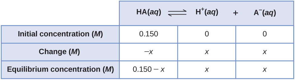
The same equilibrium concentrations are achieved whether we start with all (or mostly) reactants or start with all (or mostly) products. For example, consider the ionization of 0.150 M HA, a weak acid:
The most obvious way to determine the equilibrium concentrations would be to start with only reactants. This can be called the “all reactant” starting point. Using x for the concentration of acid ionized at equilibrium, the ICE table is
Substituting the equilibrium concentrations into the equilibrium constant equation:
gives the quadratic equation:
Solving for x using the quadratic formula:
The second solution is physically impossible because it involves negative equilibrium concentrations. Using the positive (physically reasonable) root, the equilibrium concentrations are
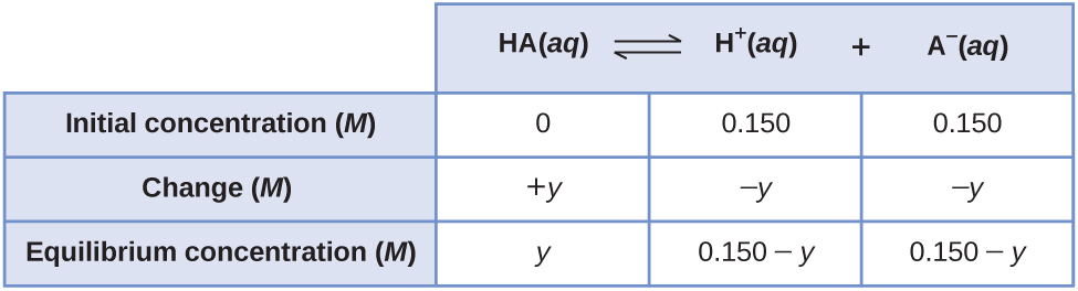
We can also solve the problem assuming all the HA ionizes first, and then the system comes to equilibrium. This can be called the “all product” starting point:
Using these as initial concentrations and “y” to represent the concentration of HA at equilibrium, the ICE table is
Substituting into the equilibrium constant equation and solving for y:
Retain a few extra significant figures to minimize rounding problems:
The first root would give an equilibrium concentration of HA that is larger than 0.150 M, which is physically unreasonable. Using the physically reasonable root (0.140) gives the equilibrium concentrations as:
Thus, the two approaches give the same results (to three decimal places), and show that starting with all products leads to the same equilibrium conditions as starting with all reactants. (Note that this is true only if the same total amount of atoms is present in both cases. Here we started with 0.150 M HA or with 0.150 M H+ and 0.150 M A−. Had we started with 0.140 M H+ and 0.160 M A−, the equilibrium concentrations would not be the same.)
The “all reactant” starting point resulted in a relatively small change (x) because the system was close to equilibrium, while the “all product” starting point had a relatively large change (y) that was nearly the size of the initial concentrations. Thus, we see that a reaction that starts “close” to equilibrium will require only a ”small” change in conditions to reach equilibrium. We can utilize this to find solutions to equilibrium problems without actually solving a quadratic (or more complicated) equation.
Recall that a very small Kc means that very little of the reactants form products and a very large Kc means that most of the reactants form products. If the system can be arranged so it starts “close” to equilibrium, then any change in concentration that is small compared to the initial concentrations can be neglected. Small is usually defined as resulting in an error that does not change the answer given the significant figures involved.
Here is an example of a calculation where the equilibrium favors products:
Given that 0.010 mol Cu2+ is added to 1.00 L of a solution of 1.00 M NH3, we can find the equilibrium concentrations.
The equilibrium constant is very large so it would be better to start with as much product as possible because “all products” is much closer to equilibrium than “all reactants.” Note that Cu2+ is the limiting reactant; if all 0.010 M of it reacts to form product the concentrations would be:
Using these values as initial concentrations, the ICE table is:
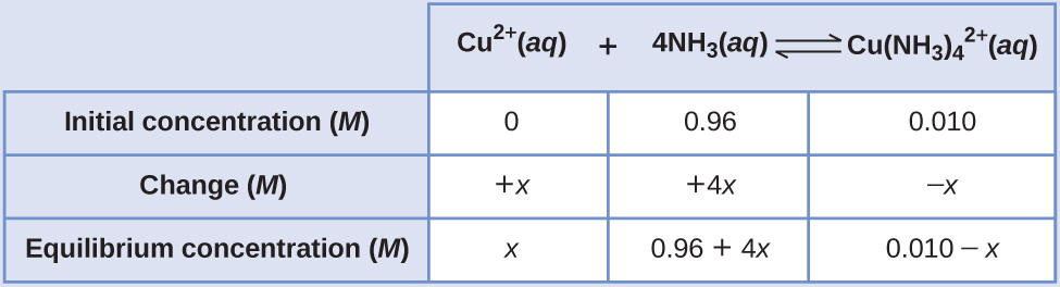
Since we are starting close to equilibrium, x should be small so that:
This is much less than 0.010 M, so the approximations are valid. The concentrations at equilibrium are:
Thus, we avoided having to solve a fifth order polymonial function, and the result is valid and well within the given significant figures.
D29.4 Reaction Quotient
We can write the reaction quotient (Q) for a generic reaction:
as:
In Qc the subscript “c” indicates Q is in terms of concentrations; we could write Qp similarly in terms of partial pressures. The concentrations are represented by “(concC)” to emphasize that Qc for a reaction depends on the concentrations present at the time when Qc is determined. These are usually not equilibrium concentrations, but they can be equilibrium concentrations if Qc is determined after equilibrium has been achieved. When only reactants are present, Qc = 0. As the reaction proceeds, Qc increases because product concentrations increase and reactant concentrations decrease (Figure 1). When the reaction reaches equilibrium, Qc no longer changes because the concentrations no longer change, and, at equilibrium, Qc = Kc.
![Three graphs are shown and labeled, “a,” “b,” and “c.” All three graphs have a vertical dotted line running through the middle labeled, “Equilibrium is reached.” The y-axis on graph a is labeled, “Concentration,” and the x-axis is labeled, “Time.” Three curves are plotted on graph a. The first is labeled, “[ S O subscript 2 ];” this line starts high on the y-axis, ends midway down the y-axis, has a steep initial slope and a more gradual slope as it approaches the far right on the x-axis. The second curve on this graph is labeled, “[ O subscript 2 ];” this line mimics the first except that it starts and ends about fifty percent lower on the y-axis. The third curve is the inverse of the first in shape and is labeled, “[ S O subscript 3 ].” The y-axis on graph b is labeled, “Concentration,” and the x-axis is labeled, “Time.” Three curves are plotted on graph b. The first is labeled, “[ S O subscript 2 ];” this line starts low on the y-axis, ends midway up the y-axis, has a steep initial slope and a more gradual slope as it approaches the far right on the x-axis. The second curve on this graph is labeled, “[ O subscript 2 ];” this line mimics the first except that it ends about fifty percent lower on the y-axis. The third curve is the inverse of the first in shape and is labeled, “[ S O subscript 3 ].” The y-axis on graph c is labeled, “Reaction Quotient,” and the x-axis is labeled, “Time.” A single curve is plotted on graph c. This curve begins at the bottom of the y-axis and rises steeply up near the top of the y-axis, then levels off into a horizontal line. The top point of this line is labeled, “k.”](https://wisc.pb.unizin.org/app/uploads/sites/126/2017/08/CNX_Chem_13_02_quotient.jpg)
A system that is not at equilibrium proceeds in the direction that establishes equilibrium (Qc changes until it equals Kc). Hence, we can predict directional shifts of a reaction by comparing Qc and Kc: when Qc < Kc, the reaction will proceed to the right (product side); when Qc > Kc, the reaction will proceed to the left (reactant side).
For example, for this reaction:
different starting mixtures of CO, H2O, CO2, and H2 will react to reach compositions corresponding to the same value of Qc; that is, will proceed until Qc = Kc (Figure 2).
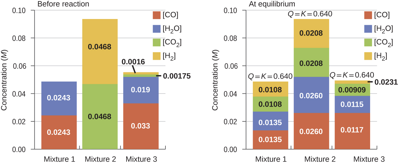
It is important to recognize that the same equilibrium value of Qc is established starting from all reactants, all products, or a mixture of both. In fact, one technique to determine whether a reaction is truly at equilibrium is to start with only reactants in one experiment and start with only products in another. If the same value of the reaction quotient is observed when the concentrations stop changing in both experiments, then we may be certain that the system has reached equilibrium.
Example 6
Predicting the Direction of Reaction
Given here are the starting concentrations of reactants and products for three experiments involving the reaction:
Determine in which direction the reaction proceeds as it goes to equilibrium in each of the three experiments.
| Reactants/Products | Experiment 1 | Experiment 2 | Experiment 3 |
|---|---|---|---|
| (concCO)initial | 0.0203 M | 0.011 M | 0.0094 M |
| (concH2O)initial | 0.0203 M | 0.0011 M | 0.0025 M |
| (concCO2)initial | 0.0040 M | 0.037 M | 0.0015 M |
| (concH2)initial | 0.0040 M | 0.046 M | 0.0076 M |
Solution
Experiment 1:
Qc < Kc (0.039 < 0.64) so the reaction shifts to the right.
Experiment 2:
Qc > Kc (140 > 0.64) so the reaction shifts to the left.
Experiment 3:
Qc < Kc (0.49 < 0.64) so the reaction shifts to the right.
Check Your Learning
Calculate the reaction quotient and determine the direction in which each of the following reactions will proceed to reach equilibrium.
(a) A 1.00-L flask containing 0.0500 mol of NO(g), 0.0155 mol of Cl2(g), and 0.500 mol of NOCl:
(b) A 5.0-L flask containing 17 g of NH3, 14 g of N2, and 12 g of H2:
(c) A 2.00-L flask containing 230 g of SO3(g):
Answer:
(a) Qc = 6.45 × 10³ M−1, shifts right. (b) Qc = 0.23 M−2, shifts left. (c) Qc = 0 M, shifts right.
Podia Question
HCN is a weak acid that ionizes to form H+ and CN− ions. Calculate all equilibrium concentrations for a 0.15-M solution of HCN. Don’t solve a quadratic equation; rather, use an approximation method and show that the approximation is justified.
Two days before the next whole-class session, this Podia question will become live on Podia, where you can submit your answer.
