D25.2 Effect of Temperature on Equilibrium

Jia Zhou; John Moore; Etienne Garand

D25.2 Effect of Temperature on Equilibrium

Recall that:

Δ_rG° = Δ_rH° – TΔ_rS° and Δ_rG° = −RT(lnK°)

Therefore:

−RT(lnK°) = Δ_rH° – TΔ_rS°

This equation can be used to calculate K° at different temperatures, if we assume that Δ_rH° and Δ_rS° for a reaction have the same values at all temperatures. This is a good, but not perfect, assumption. It is not a good assumption if there is a phase change for a reactant or a product within the temperature range of interest.

Dividing both sides of the equation by -RT gives:

lnK°	=	$-\dfrac{{\Delta}_rH^{\circ}}{R}\left(\dfrac{1}{T}\right)$	+	$\dfrac{{\Delta}_rS^{\circ}}{R}$
y	=	mx	+	b

A plot of lnK° vs. $\frac{1}{T}$ is called a van’t Hoff plot. The graph has a slope of $-\frac{{\Delta}_rH^{\circ}}{R}$ . Therefore, if the concentrations of reactants and products are measured at various temperatures so that K° can be calculated at each temperature, the reaction’s Δ_rH° can be obtained from a van’t Hoff plot.

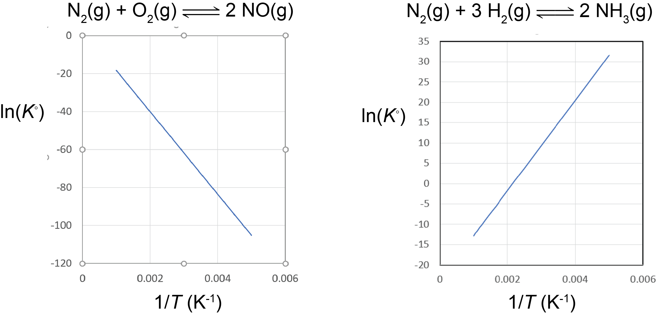
**Figure: Van’t Hoff plots**. The reaction N₂ + O₂ ⇄ 2 NO has Δ_rH° = 180.5 kJ/mol. For this endothermic reaction, as T increases (1/T decreases) the equilibrium constant increases. The reaction N₂ + 3 H₂ ⇄ 2 NH₃ has Δ_rH° = −92.2 kJ/mol. For this exothermic reaction, as T increases (1/T decreases) the equilibrium constant decreases.

Based on the equation for the van’t Hoff plot, an exothermic reaction (Δ_rH° < 0) has K° decreasing with increasing temperature, and an endothermic reaction (Δ_rH° > 0) has K° increasing with increasing temperature. The magnitude of Δ_rH° will dictate how rapidly K° changes as a function of temperature.

For example, suppose that K°₁ and K°₂ are the equilibrium constants for a reaction at temperatures T₁ and T₂, respectively:

$\text{ln}K_1^{\circ} = -\dfrac{{\Delta}_{\text{r}}H^{\circ}}{R}\left(\dfrac{1}{T_1}\right)\;+\;\dfrac{{\Delta}_{\text{r}}S^{\circ}}{R}$

$\text{ln}K_2^{\circ} = -\dfrac{{\Delta}_{\text{r}}H^{\circ}}{R}\left(\dfrac{1}{T_2}\right)\;+\;\dfrac{{\Delta}_{\text{r}}S^{\circ}}{R}$

Subtracting the two equations yields:

$\begin{array}{rcl}\text{ln}K_2^{\circ}\;-\;\text{ln}K_1^{\circ} &=& \left(-\dfrac{{\Delta}_{\text{r}}H^{\circ}}{R}\left(\dfrac{1}{T_2}\right)\;+\;\dfrac{{\Delta}_{\text{r}}S^{\circ}}{R}\right) - \left(-\dfrac{{\Delta}_{\text{r}}H^{\circ}}{R}\left(\dfrac{1}{T_1}\right)\;+\;\dfrac{{\Delta}_{\text{r}}S^{\circ}}{R}\right)\\[1em] \text{ln}\left(\dfrac{K_2^{\circ}}{K_1^{\circ}}\right) &=& -\dfrac{{\Delta}_{\text{r}}H^{\circ}}{R}\left(\dfrac{1}{T_2}\;-\;\dfrac{1}{T_1}\right)\\[1em] \text{ln}\left(\dfrac{K_2^{\circ}}{K_1^{\circ}}\right) &=& \dfrac{{\Delta}_{\text{r}}H^{\circ}}{R}\left(\dfrac{1}{T_1}\;-\;\dfrac{1}{T_2}\right) \end{array}$

Thus calculating Δ_rH° from tabulated Δ_fH° values and measuring the equilibrium constant at one temperature would allow us to calculate the equilibrium constant at any other temperature (assuming that Δ_rH° and Δ_rS° are independent of temperature).

Using this equation, you can also estimate Δ_rH° without constructing a van’t Hoff plot if K° was determined at only two temperatures (but the result will not be as accurate as a van’t Hoff plot constructed from numerous data points).

Left-click here for different forms of the equation

You can multiply both side of the equation by -1 and obtain:

$-\text{ln}\left(\dfrac{K_2^{\circ}}{K_1^{\circ}}\right) = -\dfrac{{\Delta}_{\text{r}}H^{\circ}}{R} \left(\dfrac{1}{T_1}\;-\;\dfrac{1}{T_2}\right)$

$\text{ln}\left(\dfrac{K_1^{\circ}}{K_2^{\circ}}\right) = \dfrac{{\Delta}_{\text{r}}H^{\circ}}{R} \left(\dfrac{1}{T_2}\;-\;\dfrac{1}{T_1}\right)$

Whichever form of the equation you use, keep careful track of the subscripts on the variables K₁°, T₁, K₂°, and T₂.

Exercise: Temperature Dependence of the Equilibrium Constant

Left-click here to read more about Van’t Hoff plots and Δ_rG° vs. T relationships

You may have noticed that when a reaction is product-favored or reactant-favored at all temperatures, it appears that Δ_rG° and K° have opposite trends with respect to changes in temperature. This is a rather subtle and complex issue, and one which we will not delve deeply into in this course. But we can unravel this a little bit by considering what we already know.

The relationship between Δ_rG° and K° has a temperature dependence:

Δ_rG° = −RT(lnK°)

While Δ_rG° itself has a temperature dependence:

Δ_rG° = Δ_rH° – TΔ_rS°

and K° itself also has a temperature dependence:

$\text{ln}K^{\circ} = -\dfrac{{\Delta}_{\text{r}}H^{\circ}}{R}\left(\dfrac{1}{T}\right)\;+\;\dfrac{{\Delta}_{\text{r}}S^{\circ}}{R}$

Therefore, temperature dependence of Δ_rG° is informed by the rising impact of the entropy term (Δ_rS°). In contrast, temperature dependence of K° is informed by the shrinking impact of the enthalpy term (Δ_rH°). Usually, the two impacts point in the same direction, but this is not necessarily the case in the always product-favored or always reactant-favored situations.

Keep in mind that these temperature relationships we are discussing are simplified: we are not accounting for the possible temperature dependence of Δ_rH° and Δ_rS° terms.

Comments
Please use this form to report any inconsistencies, errors, or other things you would like to change about this page. We appreciate your comments. 🙂 (Note that we cannot answer questions via the google form. If you have a question, please post it on Piazza.)

License

Icon for the Creative Commons Attribution-NonCommercial-ShareAlike 4.0 International License

Chem 109 Fall 2023 Copyright © by Jia Zhou; John Moore; and Etienne Garand is licensed under a Creative Commons Attribution-NonCommercial-ShareAlike 4.0 International License, except where otherwise noted.