
D5.1 Forces Between Atoms
In Days 2 through 4, we have discussed atomic structure and electron density as well as periodic trends in effective nuclear charge, size of atoms, ionization energies, and electron affinities. All of these are central to understanding properties and chemical reactivity of the elements. Next, we apply those ideas to noble gases and metals.
Applying Core Ideas: Two Similar Atoms, Two Very Different Substances
The section Matter, Energy, Models introduced the idea that atoms, molecules, and oppositely charged ions attract and that their potential energy can be described by a curve that starts at zero when the particles are far apart, falls to a minimum, and increases when the particles are very close together. The depth of the minimum in such a curve can be related to physical properties such as boiling points, because atomic-level particles gain energy as temperature increases.
Consider the boiling points of the first five noble gases in the table below.
| Noble Gas | Atomic Number | Atomic Radius (pm) | Boiling Point (K) |
| He | 2 | 31 | 4.22 |
| Ne | 10 | 68 | 27.1 |
| Ar | 18 | 91 | 87.4 |
| Kr | 36 | 108 | 119.9 |
| Xe | 54 | 126 | 165 |
Based on the boiling point data, for which noble gas is the attraction between particles greatest? Which noble gas has the deepest minimum in its curve of potential energy vs distance between atoms? In your notebook, answer these questions. Then use one set of axes and sketch the potential-energy curve for each of the five noble gases in the table, describe the curves in words and explain why you drew the curves as you did.
Draw and write in your notebook, then left-click here for an explanation.
Xenon has the highest boiling point. This implies that the forces between xenon atoms are larger than the forces between other noble-gas atoms and that the minimum energy for a pair of Xe atoms is lower than for the other noble-gas atoms. Thus the potential energy curve for xenon should have the deepest minimum.
Helium should have the shallowest minimum and the minima should get deeper going from He to Ne to Ar to Kr and to Xe.
Also, because the electrons in the noble-gas atoms occupy successively larger shells going from He to Ne to Ar to Kr and to Xe, the minima should be at successively larger distances between the atoms. Bigger atoms repel at larger distances because of their larger size.
A set of potential energy curves for all of the noble gases is in the figure below. This figure is based on data from a scientific paper about the attractive forces between noble-gas atoms.
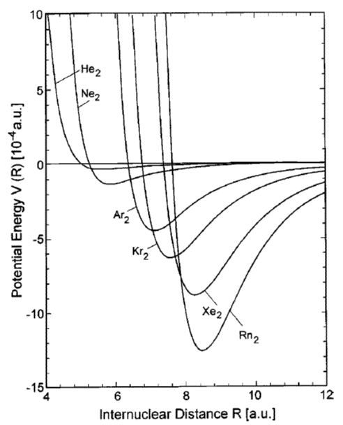
Based on the experimental data and the curves you drew, correlate the size of the attraction between atoms with the number of electrons and the size of each atom. Write several sentences in your notebook describing the correlation.
Write in your notebook, then left-click here for an explanation.
The number of electrons in an atom is the same as the atomic number: He = 2; Ne = 10; Ar = 18; Kr = 36; and Xe = 54. The sizes of the noble-gas atoms increase with the sizes of the electron shells, which also increase with atomic number and with row number in the periodic table. The largest forces between atoms (and the lowest minima in potential energy curves) are for noble-gas atoms with largest atomic number. Thus, attractive force and energy minimum correlate positively with number of electrons and with atomic radius.
Now consider iron, which has atomic number 26 and atomic radius 126 pm (the same radius as Xe, but fewer electrons). Based on this information, sketch the potential energy curve for iron atoms on the graph you made for the noble gases. Describe the curve in words and explain why you drew the curve as you did.
Does what you predicted for iron make sense?
Draw and write in your notebook, then left-click here for an explanation.
Based on the correlation of forces between noble-gas atoms with number of electrons and atomic radius, it would be reasonable to expect that the potential energy curve for iron would be similar in depth to the curve for Kr. (Fe has fewer electrons than Kr but has larger radius. Because both more electrons and larger size correlate with deeper minimum, similarity to Kr is reasonable.)
The minimum in the curve should be at a distance between atoms similar to the distance for Xe because Fe and Xe atoms are the same size.
But Fe is a solid at room temperature, not a gas, so this correlation does not work for Fe. There must be something about Fe atoms that results in much larger forces of attraction between the atoms. Our model that worked for the noble gases must be modified or a new model built to explain the properties of Fe.
Based only on experimental data for noble gases, one might predict that iron would be a gas at room temperature, but iron is a solid. Attractive forces between iron atoms must be a lot stronger than attractive forces between noble-gas atoms. To make sense of the difference between xenon and iron, we need a better model for forces between atoms.
Let’s begin by thinking about attractions between xenon atoms. On average the electron density distribution of the 54 electrons surrounding a xenon nucleus is spherically symmetric. That is, no matter which direction you go from the nucleus, the electron density is the same at the same distance from the nucleus. However, there can be very brief deviations or fluctuations from this average. In 1928, German-American physicist Fritz London used quantum mechanics to show how such fluctuations could lead to attractive forces between atoms and other atomic-scale particles.
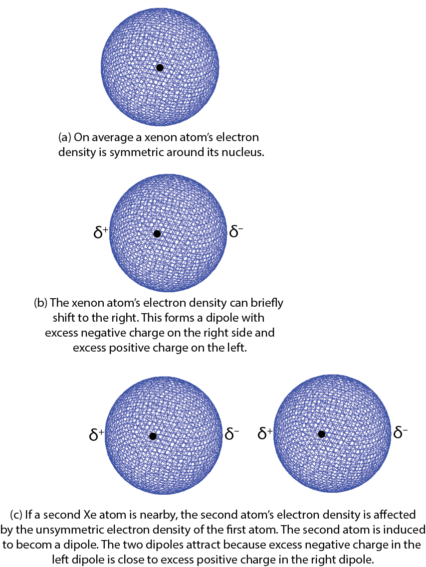
Here is a simplified explanation using Xe atoms as an example. Consider a fluctuation in which there is slightly more electron density on one side of the nucleus than on the other. Such a brief deviation creates a dipole, a distribution of electric charge where one side is more positive and the other side is more negative. This dipole only occurs for an instant and is therefore called an instantaneous dipole. This is shown in the figure part (b) at the right, where δ+ and δ− indicate a fraction of an electron’s charge.
If a second Xe atom is close to the first one when the instantaneous dipole forms, for example, in the figure part (c), the excess negative charge on the right of the first Xe atom repels the electrons on the second Xe atom. This forms a second dipole, again for only an instant. The second dipole is said to be induced by the first one. The positively charged end of the second dipole is attracted to the negatively charged end of the first dipole. For the instant that the dipoles exist, there is a weak attraction between the two atoms.
These weak attractive forces due to instantaneous fluctuations in electron density are called London dispersion forces; we will often refer to them as LDFs. LDFs are present between all atomic-scale particles: atoms, molecules, and ions. The size of the attractive force depends on the number of electrons in a particle and how easily the electron density distribution can be distorted from its average shape.
Why is an attractive force called the London “dispersion” force?
The quantum mechanical theory that Fritz London used to calculate the strength of London dispersion forces is similar to the quantum mechanical theory of light dispersion. Consequently, London called the attraction a “dispersion effect”. The term “dispersion” has nothing to do with dispersion of molecules; indeed, LDFs have exactly the opposite effect.
Think about how you could test this idea expressed in the text: LDFs are proportional to the number of electrons in an atomic-scale particle.
One way is to make a graph of boiling point (which should increase in proportion to strength of LDFs) versus number of electrons. Obtain data for boiling point and number of electrons for each of the noble gases: He, Ne, Ar, Kr, and Xe and use Excel or some other plotting software to make a graph. Does the data you used to make the graph support the statement?
Make your graph and draw conclusions, then left-click here for an explanation.
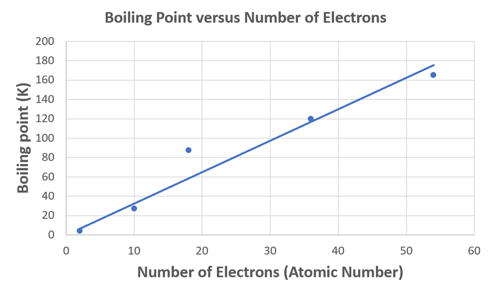
The data points are nearly on a straight line passing through the origin, which would denote direct proportionality. There are some deviations from the line, notably Ar (atomic number 18), so the generalization is not perfect. Nevertheless, the idea that LDFs increase as number of electrons increases is very useful.
Please use this form to report any inconsistencies, errors, or other things you would like to change about this page. We appreciate your comments. 🙂 (Note that we cannot answer questions via the google form. If you have a question, please post it on Piazza.)
