
D2.5 Wave-Particle Duality
The combined wave and particle model is referred to as wave-particle duality. Its impact in describing atomic-scale particles (protons and electrons) is dramatic: wave-particle duality implies that we should not just think of an electron as located at a specific position around a nucleus or moving in a specific direction and with a specific speed: the wave-like electron seems to be all around the nucleus at once! In other words, the wave nature of an electron is just as important in describing its properties as its particle nature.
An important consequence of wave-particle duality is the Heisenberg uncertainty principle: it is impossible to simultaneously determine the exact position and the exact momentum of an atomic-level particle. This means that, if we know exactly where an electron is at one instant, we have no idea where it will be an instant later; or, if we know an electron’s exact speed and direction, we have no information about where it is. As a result of the uncertainty principle, the best we can do is determine the probability of finding an electron at a specific position; that probability is proportional to the square of the wave function, ψ2.
Left-click here for optional information
For a more detailed description of the Heisenberg uncertainty principle, click here.
The electron-density distribution (or just electron density) is the three-dimensional distribution of electron probability, which can be derived from the square of a wave function. Wave functions and their electron-density distributions are called orbitals. It is these orbitals that help us understand atomic properties, chemical bonds, and forces between molecules.
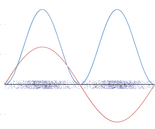
A graphic way of showing electron-density distribution (depicting an orbital) is by the density of shading or stippling. That is, we draw lots of dots or darker shading where the probability is high and we draw fewer dots where the probability is low. For example, consider the wave shown below in red along with its square shown in blue. Wherever there is a maximum in the square of the wave function (blue curve), there are many dots. Where the wave function (and therefore also its square) approaches zero, there are few dots.
Such a way to visualize electron density is quite useful for a 3-D view of the electron density surrounding a nucleus. For example, you can see the electron-density distribution of a hydrogen atom in its ground state in the video below, where the hydrogen atom is rotated around its nucleus.
In your class notebook write a description of
- The shape of the electron density distribution for a ground-state H atom
- How electron density changes with distance from the nucleus. (The nucleus is located at the intersection of the three axes: x, y, and z axes).
Write in your notebook, then left-click here for an explanation.
(1) The electron density is spherically symmetric; that is, the overall shape of the dots is roughly spherical and in any direction from the nucleus the electron density is the same at the same distance from the nucleus.
(2) The electron density decreases as distance from the nucleus increases.
In the electron-density diagram below, click on the white cross that corresponds to the lowest electron density.
Based on the density of dots in the diagram, make a graph with electron density on the vertical axis and distance from the nucleus on the horizontal axis. How is a graph of wave function versus distance from the nucleus related to the graph you made?
Draw graph and write in your notebook. Then left-click here for an explanation.
The density of dots is greatest near the nucleus and becomes smaller as distance from the nucleus increases. The graph should be highest at the nucleus and decrease with increasing distance from the nucleus. The image on the left side below shows the graph with the nucleus at the origin of the coordinates; your graph might differ but should decrease steadily the farther it goes from the nucleus.
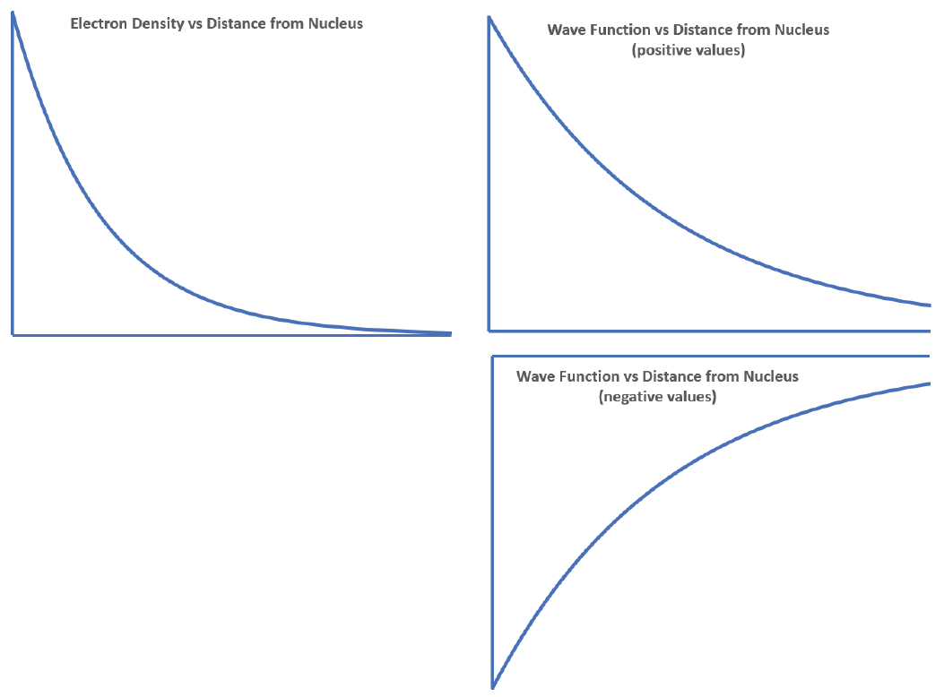
A graph of the wave function can be derived from the graph of electron density because the electron density function is the square of the wave function. Thus the wave function should decrease in magnitude the greater the distance from the nucleus. However, there is no way to tell the mathematical sign of the wave function from the electron density function. The wave function might have positive values or it might have negative values, because squaring a negative value gives a positive result. The right side below shows two possible graphs for the wave function.
Similar to dot-density diagrams, but visually simpler while conveying a little less information, are 3-D boundary-surface plots. These plots show a surface that has the same shape as the electron density distribution and encloses some fraction, such as 90%, of the electron density. That is, if we could repeatedly locate the electron exactly, nine times out of ten the electron would be located inside the boundary surface. The figure below shows how a boundary surface is related to the dot-density plot you have already viewed. Move the slider at the bottom to change from dot-density to boundary-surface diagram.
Visualizing electron-density distributions confirms an idea mentioned earlier: there are shells of electron density, concentric spheres each farther from the nucleus. The orbitals that belong to a given shell have the same quantum number, n, and their electron density is approximately the same average distance from the nucleus. The principal quantum number n dictates the overall size of the orbital.
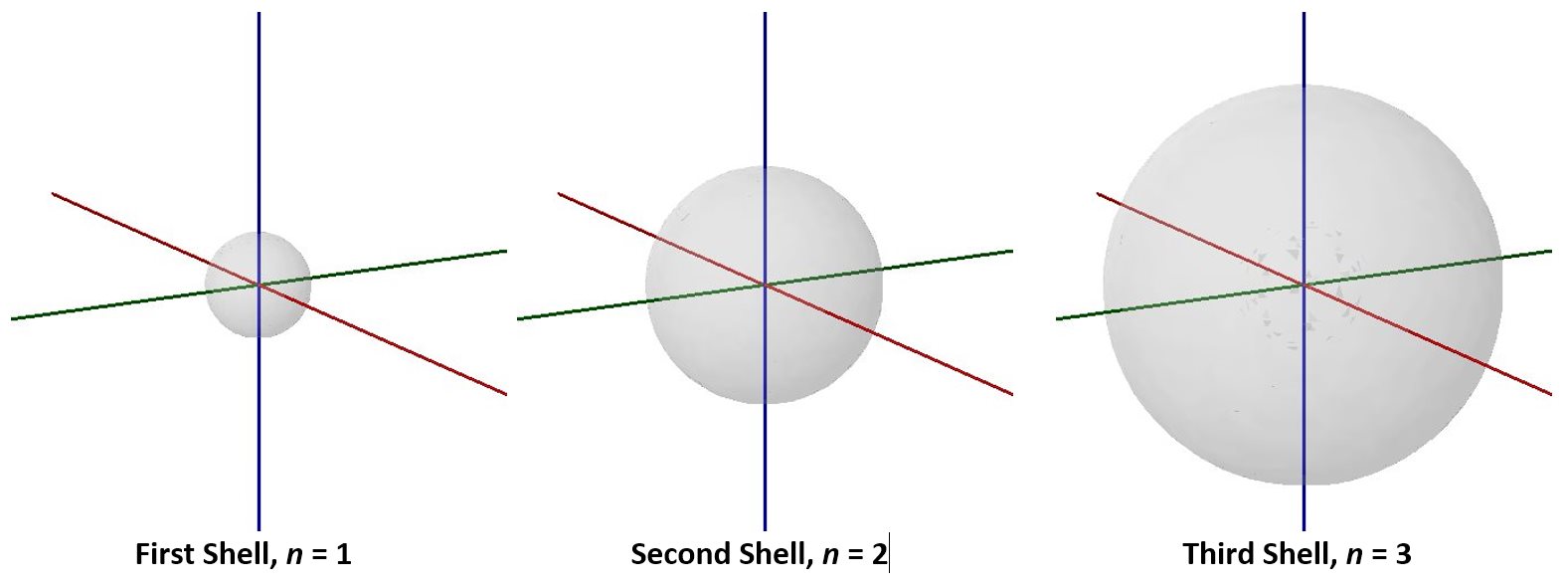
As n gets larger, the radius, r, of the electron shell gets larger, and En becomes less negative—closer to zero. Therefore, the limits n ⟶ ∞ and r ⟶ ∞ imply that En = 0 corresponds to ionization of the atom, complete separation of the electron from the nucleus. Thus, for a hydrogen atom in the ground state, the ionization energy is:
 = k = 2.179 × 10⁻¹⁸ J
Another interesting aspect is that while we know En, which is the total energy of the electron, we cannot measure the electron’s kinetic energy (or its velocity) and potential energy separately. We know from Coulomb’s law that the potential energy changes as a function of r. Since the electron density is distributed over a range of r, there’s a range of potential energy, and hence a range of kinetic energy—when the electron’s potential energy is higher, its kinetic energy would be lower. This uncertainty is again related to the wave nature of the electron. However, knowing the total energy, En, is quite sufficient for us!
Activity: Wrap-up for Atomic Spectra and Atomic Structure
Please use this form to report any inconsistencies, errors, or other things you would like to change about this page. We appreciate your comments. 🙂 (Note that we cannot answer questions via the google form. If you have a question, please post it on Piazza.)
