1

Welcome to Conservation GIS

Land Use and Landscape Change Lesson

In the following topics of this lesson, you will:

• Review basics of earth imaging for use in Conservation GIS
• Link remote sensing images to features on the ground
• Learn how to match land cover data and classifications to habitat needs of wildlife
• Explore how land use and land cover can be evaluated for conservation planning
• Apply spatial analyst to evaluate landscape change over time
• Explore other raster-based tools to capture temporal dynamics

Earth Imaging & Land Cover Data

Basics of Remote Sensing

A working knowledge of earth imaging, or remote sensing is needed to begin Conservation GIS, since it forms the basis for most land cover, and subsequently, habitat assessments.

Earth images give photo-realistic views of the Earth’s surface that can offer richer information and interpretation for many environmental applications than other forms of cartographic representation such as vector and grid data.

Some of the earliest aerial photography was conducted with the use of balloons and pigeons carrying cameras. Aerial images have been used as backdrops in GIS for decades (Fox 2015).

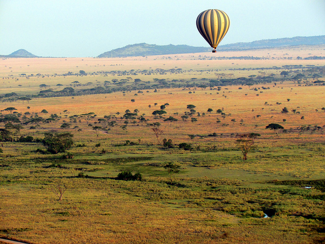
Earth imaging grew out of aerial photography as early as the 1940s, and photogrammetry and satellite imagery in the 1950s-60s. From there, the term Remote Sensing was used to mean multiple platforms, sensors, and wavelengths used to capture the Earth. More recently we include laser scanners (LiDAR), hyperspectral imagery, and unmanned aircraft among earth imaging or environmental sensing technologies (Brown and Harder 2016).

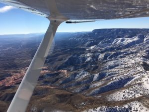
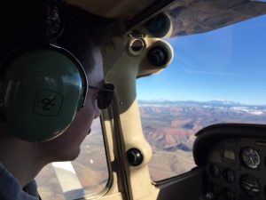
Remote sensing is “the science and art of obtaining information about an object, area, or phenomenon through the analysis of data acquired by a device that is not in contact with the object, area, or phenomenon under investigation” (Lillesand et al. 2015).

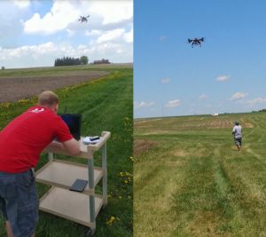
Today, remote sensing data is generated on platforms such as satellites, aircraft, and most recently, unmanned aerial systems (UAS), or drones. These platforms carry a variety of sensors, from simple color digital cameras to ground penetrating radar systems. For a nice synopsis, watch this 7 minute video with Esri’s Lawrie Jordan on the future of imagery in GIS:

https://www.esri.com/videos/iframe?videoid=5127&isLegacy=true

Remotely-sensed earth observation, or imagery, is the definitive visual reference in GIS (Brown and Harder 2016). The phrase, ‘imaging GIS’ is used by Fox (2015, p.1) to “describe a geographic information system (GIS) that displays, enhances, and facilitates the analysis of earth images.”

Basics of Remote Sensing

All surfaces reflect, absorb, or transmit energy, many within and beyond the visible spectrum (390-700nm wavelengths) into shortwave infrared and ultraviolet wavelengths.
Remote sensors are designed to measure and record reflected radiation in specific sections, or bands, of the spectrum. The pattern of reflectance in these bands provides information about objects on the ground, from their visible characteristics to moisture content and even subsurface features.

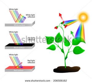
Passive sensors measure radiation that is naturally reflected (such as sunlight) or produced in the environment (such as infrared) by constituents of the Earth’s surface and its atmosphere. It is passive because the sensor does not generate its own radiation. Earth features reflect different parts of the electromagnetic (EM) spectrum at different rates, giving us spectral signatures to distinguish, for example coniferous from deciduous trees.

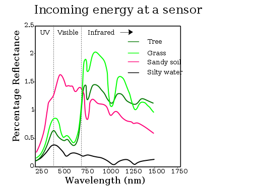
More specifically, living green plants reflect radiation in the middle of the visible spectrum at 0.45-0.6 micrometers (and thus appear green), and in the near-infrared portion of the EM spectrum. Water, on the other hand, reflects radiation in the shortest visible wavelengths, while bare soil reflects strongly across wavelengths, especially in the visible red and near-infrared bands, making it appear reddish-brown to us.

The figure below provides spectral reflectance curves for bare soil, green vegetation, and water. Measuring reflectance within discrete intervals corresponding to these peaks and valleys forms the basis for land cover classification with passive remote sensing data.

Active sensors transmit pulses of electromagnetic radiation and measure their reflection, refraction, or scatter by the Earth’s surface and atmosphere.

Active remote sensing often uses imaging radar systems that generate pulses of microwave radiation that travels to the Earth’s surface. The radiation that reflects back to the sensor is measured and can be transformed into an image. Since radar is an active system and uses very long energy waves that penetrate clouds, radar systems can capture an image even on dark rainy nights. Similarly, LiDAR systems actively create and emit their own radiation and measure how much radition reflects back from the surface. LiDAR systems can produce three dimensional data that provide elevation models for the areas captured.

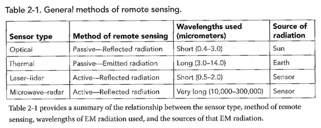
Linking earth imaging with vegetation on the ground

To interpret what is on the ground from imagery, we need to consider four attributes of images, regardless of the sensor or technology used to produce them. These four R’s refer to different characteristics of resolution that allow practitioners to determine the usefulness of images for certain applications. Of the four: spatial resolution, spectral resolution, radiometric resolution, and temporal resolution, we will focus on all but radiometric here.

Spatial Resolution refers to the spatial dimensions of an object, characterized by both grain and extent.

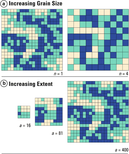
• Grain – the size of the smallest homogeneous unit of study and determines the resolution at which a landscape is studied. It is equivalent to minimum mapping unit in cartography. A pixel in a digital image is analogous to a grain in a landscape.
• Extent – the overall area included in an investigation or the area within the landscape boundary. Extent refers to both the physical area as well as the length of time for which a landscape or population process occurs.

Cartographic scale is the degree of spatial reduction indicating the length used to represent a larger unit of measure; one unit of distance on a map, aerial photograph, etc. that represents a specific unit of distance on the ground. Scale is often presented as a fraction (1/25,000) or ratio (1:25,000), where 1 inch on the map represents 25,000 inches on the ground. Subsequently, 1:25,000 defines a smaller scale and provides less detail than 1:10,000 (larger scale). More often in ecology however, use of large and small scale is transposed (Silbernagel 1997).

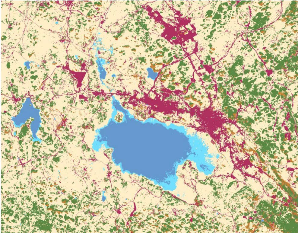
Spectral Resolution

To capture features on the Earth’s surface, remote sensors detect ranges of wavelengths in the electromagnetic radiation (EM) emitted by the sun and Earth. Even a basic camera or GoPro on a drone captures spectral radiation in the visible wavelengths with optical sensors.
The number and width of bands recorded by a sensor defines the spectral resolution of the data. Some sensors collect ‘hyperspectral’ imagery, meaning they can capture many narrow bands of the spectrum (5-10 nm), whereas, multispectral imagery is usually composed of 5-10 bands of relatively large bandwidths (70-400 nm).

The combination of reflectance in the visible and invisible ranges of different kinds of landcover can be fine-tuned into spectral signatures that can distinquish between types of plants, aquatic and upland ecosystems, or healthy and diseased forests.
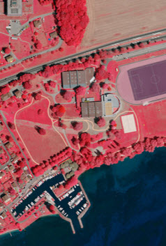
For example, vegetation reflects strongly in the near infraredpart of the spectrum (wavelengths between ~700-1500 nm (corresponding to the plateau between .7 to 1.5 micrometers for the vegetation line in the graph above). The image below from the Swiss Federal Office of Topography shows how vegetation appears bright red in contrast to the tilled field, sports field, and water in this near-infrared (NIR) image.

Temporal resolution

refers to the amount of time between repeat coverage of the same area by the remote sensor. It is important to collect data from the same area on multiple dates for better classification and for change detection. In other words, the more frequently images are collected, the finer the temporal resolution, and the greater the ability to capture change on the ground. For example, Landsat 8 images the entire earth every 18 days. This represents the minimum temporal resolution for this satellite.

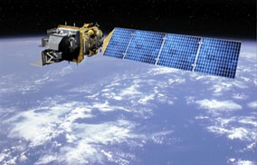
Freely available sources of satellite imagery are provided here: https://gisgeography.com/free-satellite-imagery-data-list/

Image processing and delineation of earth features, including land cover classification, is beyond the scope of this lesson. However, you will have the opportunity to display and enhance multispectral imagery in the lab exercise.

Matching the needs of wildlife with land cover data

This section describes the requirements of land cover data for developing accurate habitat models.
Vegetative requirements of wildlife can be floristic, structural, or a combination of the two. For example, the fisher generally avoids open areas and utilizes a range of plant communities containing high amounts of vegetative structure, while sage grouse are strongly associated with sagebrush habitat but also require specific structural components of sagebrush and herbaceous cover.

Because the fisher and sage grouse are habitat specialists, developing habitat models for these species requires land cover data that captures both the species composition and structure of vegetation.

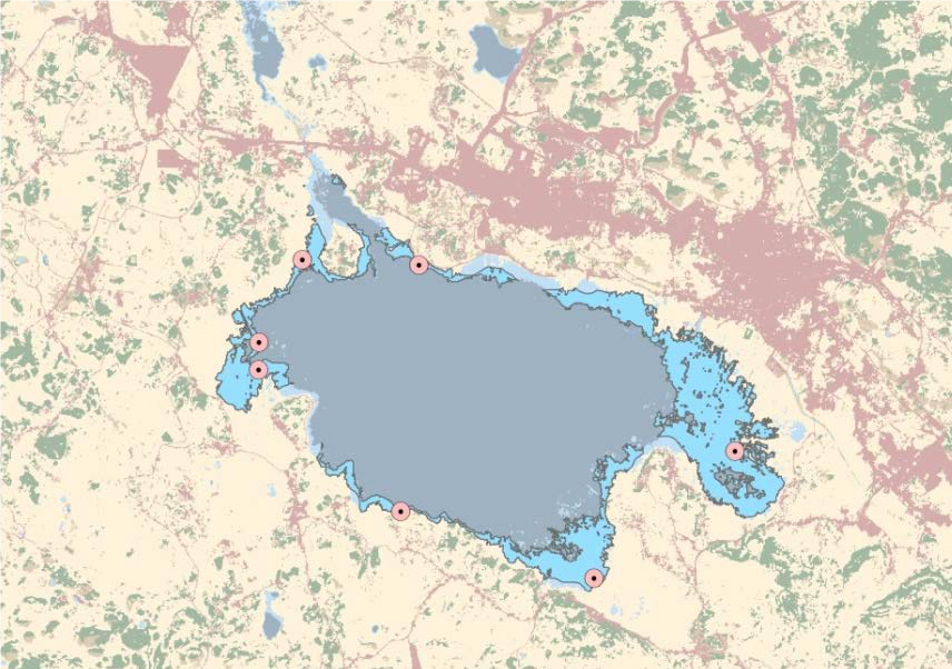
Existing land cover classifications may not adequately capture the land cover characteristics that determine habitat requirements of all species of interest. For example, a focal species such as black-necked crane, may require specific kinds of wetland habitats or water depths for foraging, yet typical land cover classifications may not distinguish among wetland types. Broader classifications of wetlands vs. uplands would overestimate the amount of suitable habitat. Likewise, classification errors, or inaccuracies – where a set of pixels are misclassified as land cover types that differ from what is on the ground – can potentially compound data limitations.

Selection of Land Cover Data

It can also be difficult to find consistent land cover data across jurisdictional boundaries that are common in conservation planning. Following are some sources of commonly available land cover data and examples of other options for classification. Some of the benefits and associated problems of each are discussed.

Global land cover data have been available since the 1990’s. Advantages are availability and consistency worldwide, but the tradeoffs are coarse resolution and very general categories. However, this is changing with the availability of Sentinel-2 data, a satellite mission led by the European Space Agency, and efforts to produce a new global land cover dataset (http://s2glc.cbk.waw.pl/project-summary).

The USGS Land Cover Institute provides a list of global land cover data sets at http://landcover.usgs.gov/landcoverdata.php. The Institute, located at the Center for Earth Resources Observation and Science (EROS) in Sioux Falls, South Dakota, works with a range of land cover products from local to global scales, and in both domestic and international settings. They help users identify suitable land cover data sets to meet research and project needs.

The USGS list also includes higher spatial resolutions and finer classifications available at a national level, most notably, the National Land Cover Database.

National Land Cover Database (NLCD)

First produced in 1992 from 1990 Landsat TM imagery (30m), updated NLCD classifications were produced in 2001, 2006, and 2011 including a landcover change map from 2001-2006. NLCD 2011was the first with the capability to assess wall-to-wall, spatially explicit, national land cover changes and trends across the United States from 2001 to 2011 at a spatial resolution of 30 meters. The latest, NLCD 2016 was released in 2019.

Advantages

• Available for the conterminous United States, Alaska, Hawaii, and Puerto Rico
• Use of 30 meter Landsat data provides good spatial heterogeneity of cover types
• Estimates of canopy coverage
• With NLCD 2016 land cover and imperviousness products will be available for 7 product dates between 2001 and 2016 including 2001, 2004, 2006, 2008, 2011, 2013, and 2016.
• Incorporation of new shrub and grass mapping in the Western U.S. is being completed.

Disadvantages

• Broad classes not well suited for delineating wildlife habitat
• Poor accuracy of some classes and locations

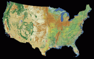
NLCD Classes

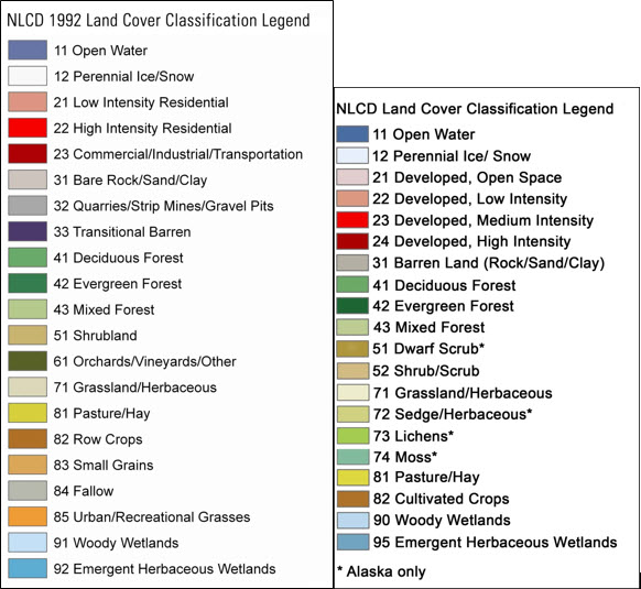
Below are the land cover classes used by the National Land Cover Dataset in 1992 vs 2001. Note that the 1992 NLCD was based on 21 classes, while today, as with two previous NLCD land cover products, NLCD 2016 uses the 16-class land cover classification scheme that has been applied consistently across the United States

Other national land cover data sets have been created for more specific applications. You were introduced to many of these earlier. Let’s take a closer look at a couple of these…

LANDFIRE Data

LANDFIRE is a program that provides over 20 national geo-spatial layers (e.g. vegetation, fuel, disturbance, etc.), databases, and ecological models that are available to the public for the US and insular areas. Vegetation is mapped using predictive landscape models based on extensive field-referenced data, satellite imagery and biophysical gradient layers using classification and regression trees. LANDFIRE uses vegetation products (e.g. maps based on land cover) to create fuel and fire regime data. Most vegetation products use NatureServe’s Ecological Systems classification, meeting the requirement that map units be identifiable, scalable, and model-able.

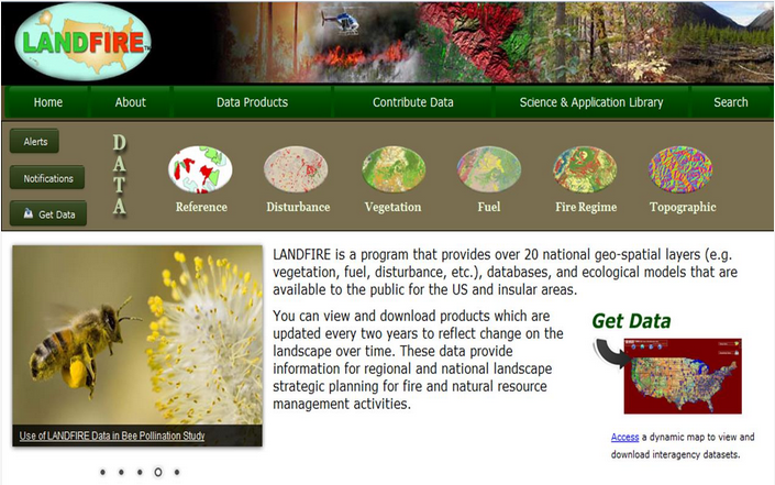
The LANDFIRE Data Access Tool is an ArcGIS toolbar that allows users to interact with the LANDFIRE Data Distribution Site and download LANDFIRE data directly into ArcMap.

LANDFIRE data is useful for:

• prioritizing fire fuel reduction
• identifying target areas for ecological restoration activities
• planning natural resource management
• mapping wildlife habitat suitability

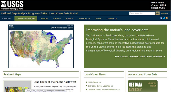
National Gap Analysis Program (GAP) Land Cover

You may recall that a Gap analysis identifies species’ habitat and distribution, protected lands in relation to those species, and where there is a ‘gap’ in protection for species. The National GAP Analsyis Program (https://gapanalysis.usgs.gov/) collects and distributes data to answer the fundamental question, “How well are protecting common plants and animals?” by identifying those species and plant communities that are not adequately represented in existing conservation lands.

Advantages

• Available for the US and Puerto Rico.
• Generally higher accuracy than NLCD due to smaller extents.
• Includes a land cover data viewer

Disadvantages

• Although the intent of GAP was to identify gaps in the protection and conservation of animal and plant species, the broad classes that are typically used often are not of sufficient accuracy to define habitat for many species.

Classification using high resolution data

High spatial resolution sensors have the potential for creating land cover classifications of smaller features that are aligned with how humans and wildlife interact with their environment. For example. IKONOS imagery, a satellite-based sensor, has shown the ability to identify tree canopy , individual trees, and to differentiate between vegetation types in dry shrub/grassland.

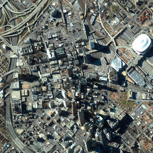However, there currently are not any widespread classifications using these types of imagery. The extent of each scene is generally small, data are fairly costly because they are produced from privately owned satellites, and the images are often taken at an angle rather than straight down. In addition, the spatial resolution provided by these sensors introduces a lot of features that are not relevant for land cover classifications, such as shadows.

High spatial resolution data is valuable in developing and validating land cover classifications because of the greater detail it provides.

1. Earth Imaging and Land Cover Data

Topic 1 Knowledge Check

Please answer the following questions to proceed to the next topic.

2. Landscape Change and Assessment

Distinguish land use from land cover

So far we have linked earth imagery to land COVER. Land cover is the biophysical state of the earth’s surface, and often refers to the dominant vegetation type present, such as forest or wetland.

Land use involves both the manner in which the biophysical attributes are manipulated and the intent underlying the manipulation. In other words, land use is the way in which and the purpose for which land is used in relation to human activities (Turner & Gardner 2015).
Examples:

• recreation (land use) on forested (land cover) land
• grazing (land use) on grassland (land cover)
• wildlife refuge (land use) on wetland (land cover)

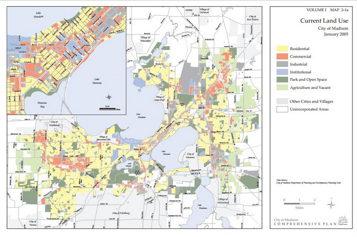
The map below shows land use for the city of Madison, Wisconsin. Follow this link to download a future land use plan of Madison.

Land use datasets

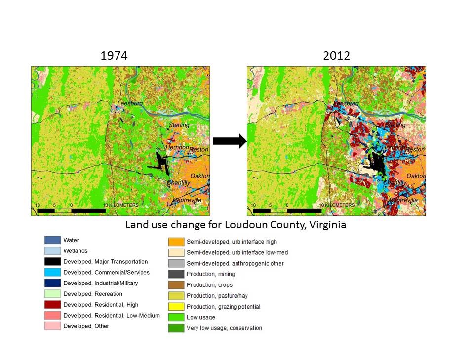
Different datasets provide different estimates of the extent of human activities because of the different purposes, sensors, and scales used to generate them. The figure below compares land use change in Loudoun County, Virginia using the U.S. Conterminous Wall-to-Wall Anthropogenic Land Use Trends (NWALT), 1974-2012.

Human Activities

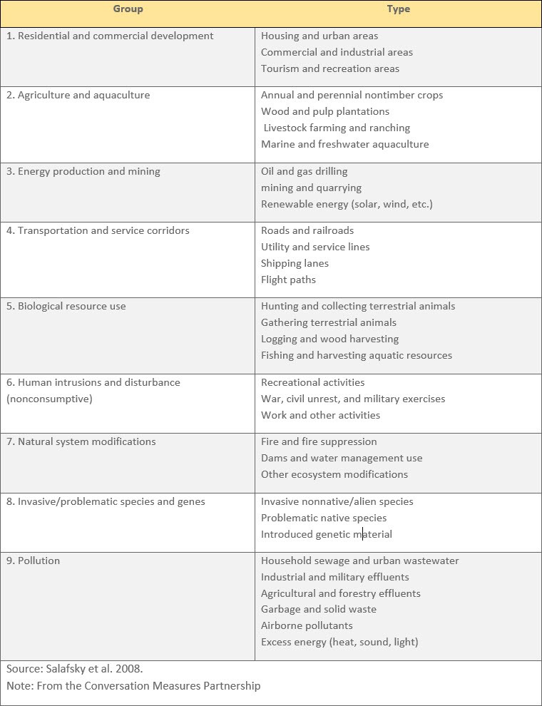
A common way to integrate land use and human modifications or land use with a conservation plan is to identify direct threats that affect or stress biodiversity targets.

The Conservation Measures Partnership created a listing of general categories of human activities that may threaten biodiversity (Salafsky et al. 2008, Table 1, http://onlinelibrary.wiley.com/doi/10.1111/j.1523-1739.2008.00937.x/full ).

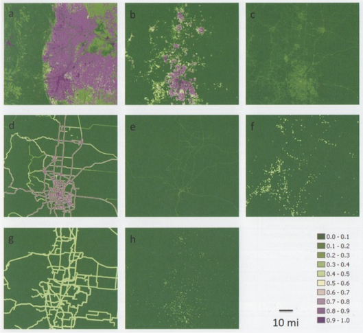
Spatial data on land use activities can be converted into indices of threat.

The figure below shows 8 different threats in the same area of the northern Front Range of Colorado–(a) degree of human modification to land cover, (b) housing density, (c) road footprint, (d) highway traffic, (e) railways, (f) mines, (g) power lines, and (h) communication and cell towers. The percentage of area within each cell modified by human activities or structures increases from dark green (0-1%) to purple (90-100%) to create a separate index of human modification for each threat. See page 115 in Craighead and Convis (2013) for a detailed explanation of how each index was calculated.

Composite index of human modification

Often multiple layers depicting separate threats will need to be simplified or combined into a single composite or cumulative index layer. We can accomplish this with weighted overlay tools in GIS.

Here, we will learn of a specific composite index for capturing the degree of human modification for conservation planning. There are many different mathematical combinations of the values for each of the threat layers in a given location, such as mean, sum or product.

In the figure below, the maps of individual indices of human modification shown on the previous page were combined using (a) maximum value, (b) mean value, and (c) fuzzy sum to create a composite index of human modification.

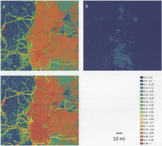
Fuzzy logic allows values and threats to belong to multiple sets of membership and does not assume complete independence among threats. For another example of how fuzzy logic can be used to map composite indices of reserve potential (areas with low human impact), view minutes 8:30-12:30 of this webinar on a conservation decision support model that uses fuzzy logic.

Projecting threats

In addition to examining current land use threats, we may want to incorporate predicted or plausible future land use into conservation planning.

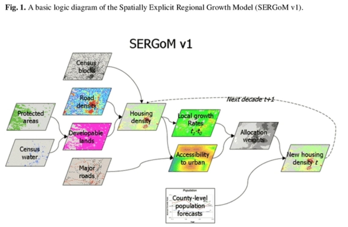
For example, Theobald (2005) used a series of land-use change models to develop a regional growth model for the US to project housing growth across US for 2030 based on population projections. Data from this Spatially Explicit Regional Growth Model (SRGoM) was used for LandScope, and is no longer publicly available.

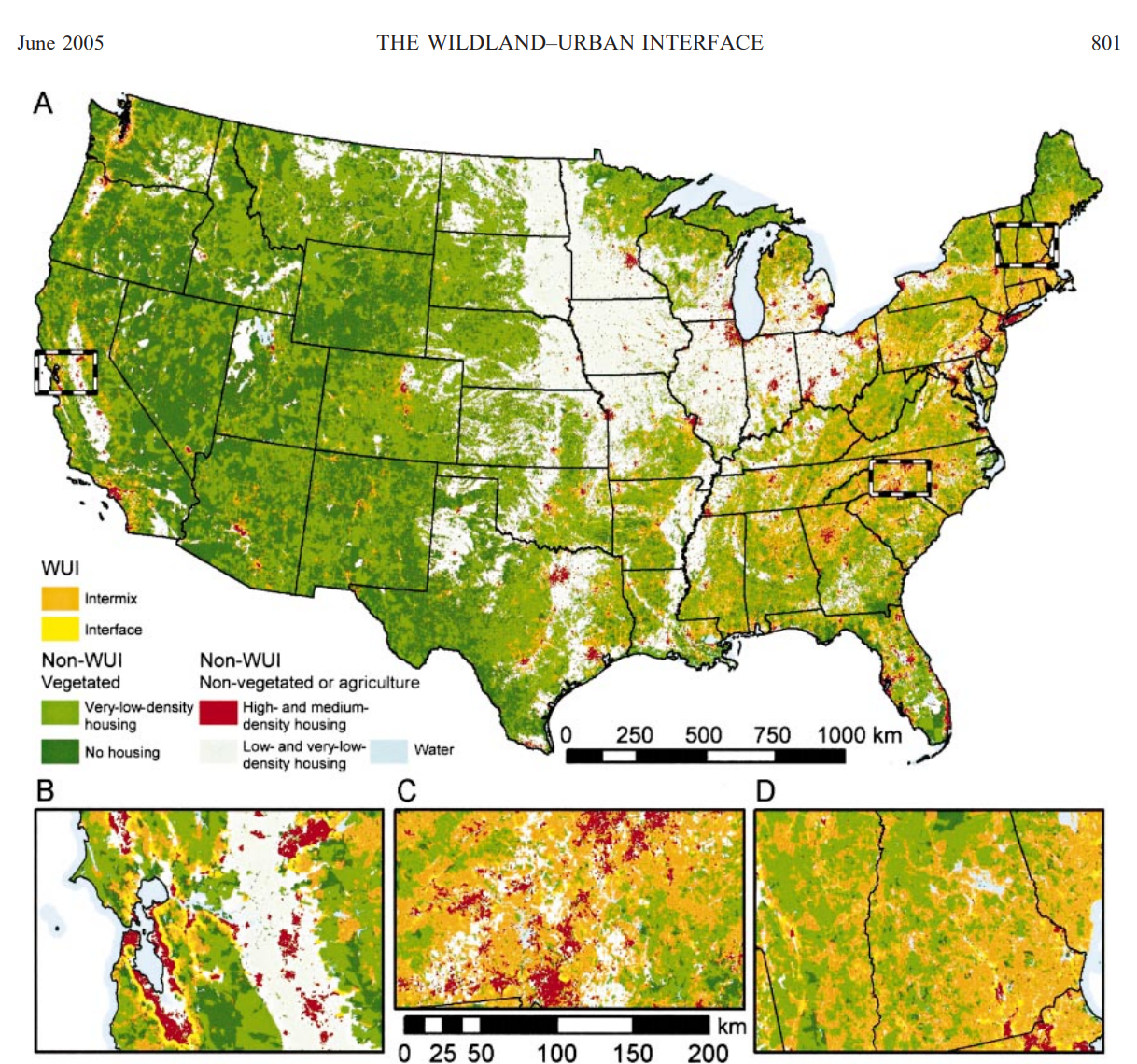
Similarly housing growth was assessed in the context of the wildland-urban interface across the US the SILVIS and Applied Population Lab at the University of Wisconsin-Madison (Radeloff et al. 2005).

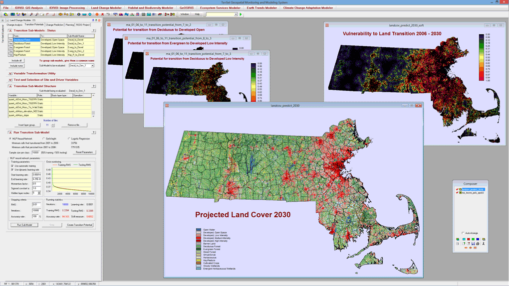
A more readily available tool for projecting landscape change, is the Land Change Modeler (LCM), which is a decision support component of TerraSet by Clark Labs, developed with support from Conservation International. LCM uses time series of spatial data, transition probabilities and complex spatial models to project change and biodiversity. We’ll take a closer look at LCM later.

Topic 2 Knowledge Check

Please answer the following questions to proceed to the next topic.

3. Spatio-temporal Analysis with Rasters

Spatio-temporal analysis

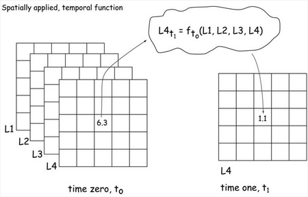
Spatio-temporal analysis involves characterizing the spatial variation of entities over time. Change in time is often described as a function (ƒ) of some set of previous conditions. Such a function not only allows us to analyze changes in land cover over time, but also enables us to project past trends into the future.

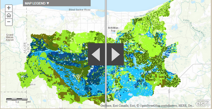
Spatio-temporal analysis is often used in land change assessment to compare two or more sequential spatial data sets. For example, the map below shows the land cover in the Two Hearted River watershed in Michigan’s Upper Peninsula today (left) and 100 years into the future if current management is continued management scenarios (right). Visit the Forest Scenarios Project website to view this map interactively.

Temporal Dynamics

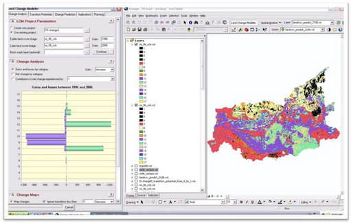
By comparing land cover or land use at multiple time points, we can get an idea of the temporal dynamics of landscapes–the ways and rates at which land cover or land use change over time. This analysis is performed by computing the difference between layers (Δ P = (P at time 2) – (P at time 1)). Models of future change can project past temporal dynamics into the future using these rates of change. For land cover, LCM builds on the concept of transition potential–the probability that a specific land cover type will transition to a different land cover type based on past trends.

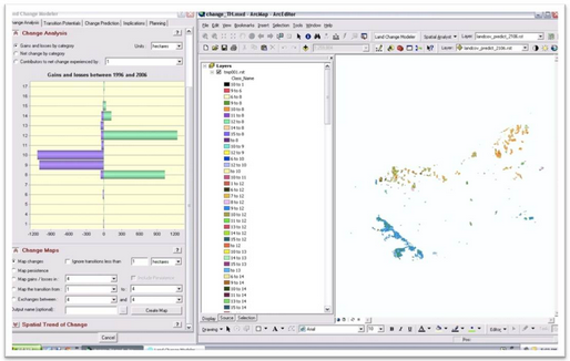It is also possible to build predictive models that involve combinations of these temporal layers related through map algebra.

There are several other useful tools for observing landscape change and performing spatio-temporal analysis.

The Landsat Time-Enabled Imagery map allows users to explore spatial data at different temporal scales and analyze change over time using web browser access.

Examples

The Swipe Layer Tool in ArcMap enables quick visualization of land change by allowing users to interactively reveal overlaid map layers. This tool makes it easy to see what is underneath a particular layer without having to turn it off in the table of contents. Swiping between two land cover layers from different times is especially useful for visualizing landscape change.

You can access the Swipe Layer tool from within the Image Analysis window, where you interact with raster layers, and you can also access it from the Effects toolbar, where you can interact with any layer in the table of contents.

Similar swipe capabilities have been built into Esri StoryMaps, which can interactively display change over time in many categories, from land use to demographics as you saw in the Forest Scenarios example.

Also from Esri, the Change Matters Viewer allows users throughout the globe to quickly view Landsat imagery both multi-spectrally (in different Landsat band combinations) and multi-temporally (across epochs) to display changes in vegetation over time.

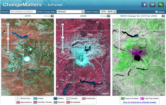
While the examples so far only visualize differences over time, the Difference Tool in Image Analysis in ArcMap allows users to quantify differences between land cover data sets.

For a more robust change analysis, clicking the Difference  button performs a basic change detection algorithm by computing the difference between two raster or image service layers. This tool can be used to compare classified images, elevation models, and more.

Beyond these basic imagery tools in ArcMap, ArcGIS Pro has an image analysis extension, https://blogs.esri.com/esri/arcgis/2018/01/08/coming-soon-image-analyst-extension/. For more robust spatio-temporal analysis, users will turn to other products like LCM, the image processing software ENVI, or writing custom functions in languages like Python and R.

Knowledge Check

Please answer the following questions to complete lesson 1

References:

Brown, Clint and Christian Harder. 2016. The ArcGIS Imagery Book: New View. New Vision. Esri Press. www.thearcgisimagerybook.com

Craighead, Lance and Charles Convis. 2013. Conservation Planning. Esri Press. chapters 4 and 5.

Fox, Lawrence. 2015. Essential Earth Imaging for GIS. Esri Press, chapters 1, 2, and 4.

Lillesand, Thomas M. and Kiefer, Ralph, W. 1994. Remote Sensing and Image Interpretation. 

RADELOFF, V. C., R. B. HAMMER, S. I. STEWART, J. S. FRIED, S. S. HOLCOMB, AND J. F. MCKEEFRY. 2005. THE WILDLAND–URBAN INTERFACE IN THE UNITED STATES. Ecological Applications, 15(3), 2005, pp. 799–805

SALAFSKY, N., SALZER, D., STATTERSFIELD, A. J., HILTON-TAYLOR, C., NEUGARTEN, R., BUTCHART, S. H. M., COLLEN, B., COX, N., MASTER, L. L., O’CONNOR, S. and WILKIE, D. (2008), A Standard Lexicon for Biodiversity Conservation: Unified Classifications of Threats and Actions. Conservation Biology, 22: 897–911. doi:10.1111/j.1523-1739.2008.00937.x

Theobald, David M. 2005. Landscape Patterns of Exurban Growth in the USA from 1980 to 2020. Ecology and Society. Vol. 10, No. 1