2 Lesson 2
Landscape Evaluation and Metrics Lesson
In this lesson, you will:
- Understand why methods for quantifying spatial pattern are necessary tools for landscape evaluation
- Learn key considerations for comparative landscape analysis that include:
- Describing how a landscape has changed through time
- Determining how patterns in two or more landscapes differ from one another
- Evaluating alternative strategies
- Making future projections regarding landscape change
- Measure components of spatial data with landscape metrics
- Apply landscape metrics through practical examples
Lesson Topics
This lesson will cover three topics and take approximately 50 minutes to complete. We recommend working through each topic in the order in which they are listed below.
The Case for Measuring Landscape Pattern
Why quantify landscape pattern?
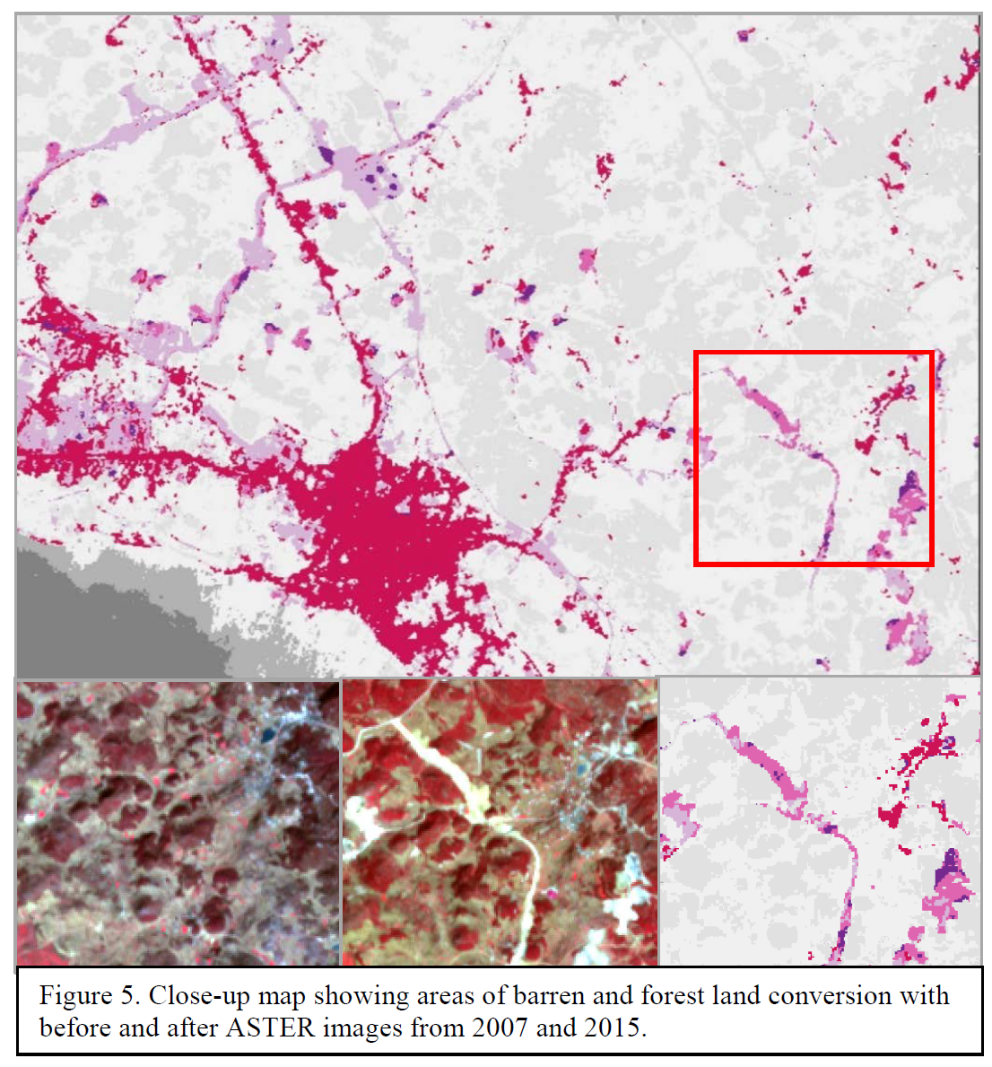
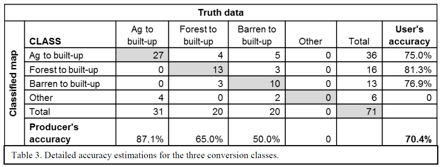
Quantifying landscape pattern allows us to compare land cover classes within the same landscape at different times. For example, with the following classified imagery, we calculated land cover type conversions at Cao Hai Lake in western China, between 2007 and 2015.
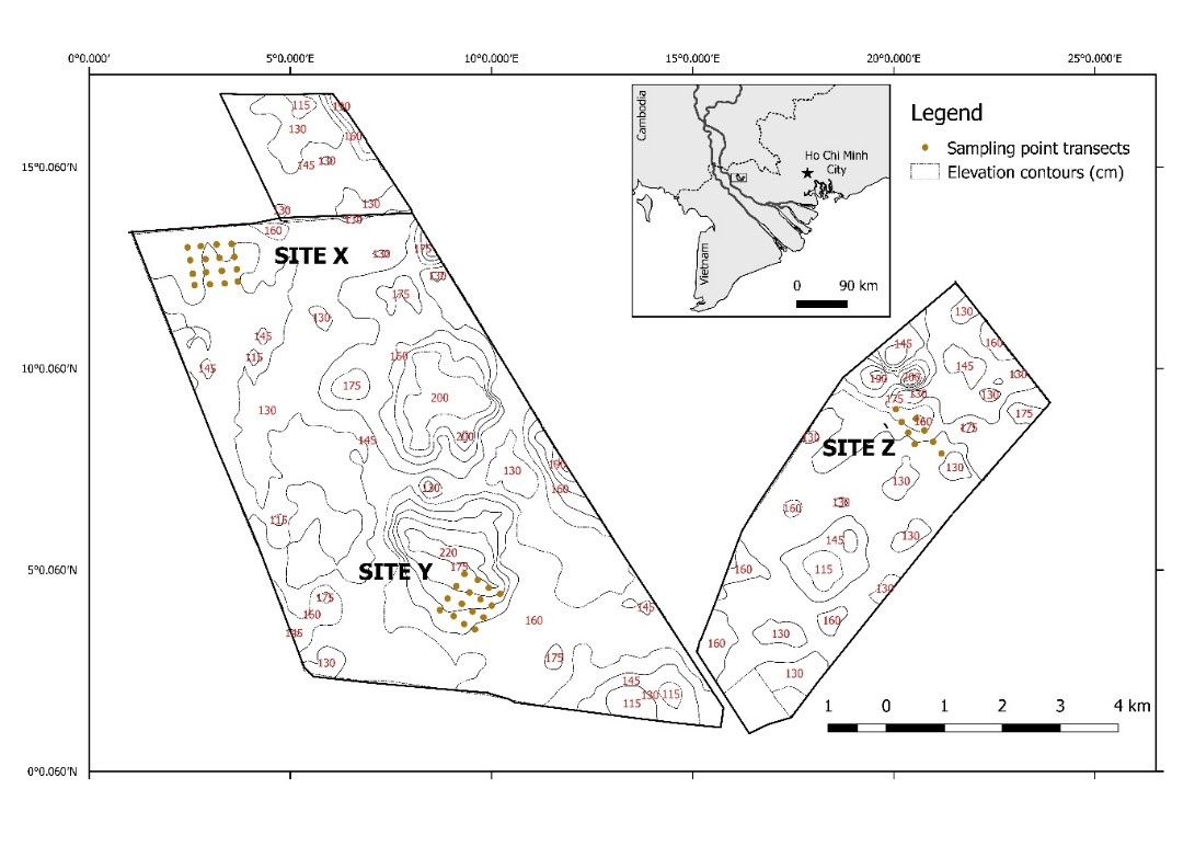
Quantifying landscape pattern also allows us to compare land cover classes among different landscapes at the same time. In the Vietnamese park example below, we quantified vegetation structure and avian communities among the three sites with different terrain, and over three different management regimes from 1996 to 2016.
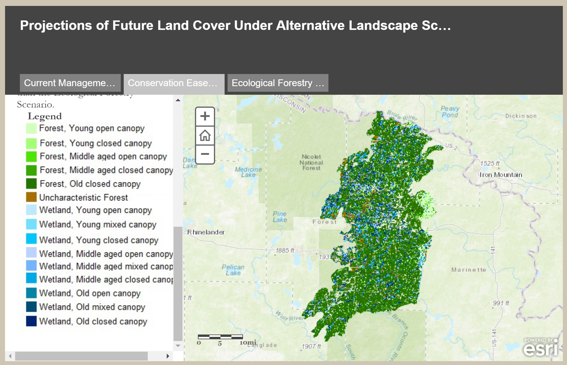
We can also compare the outcomes of different scenarios by quantifying aspects of landscape structure and how they differ between scenarios. We might ask, for instance, if wetland classes are more aggregated in a conservation-oriented scenario compared to current management.
This example compares projected vegetation structure between three different scenario outcomes for the Wild Rivers study area in northern Wisconsin.
Considerations
When comparing two or more spatial data sets we need to consider several aspects of the data. First, do the data sets have matching classification schemes? If not, consider how the data can be compared.
Below is an example of how the same landscape looks very different under different classification schemes. Both show a 5×5 km section of southwestern Yellowstone National Park, where the landscape is (a) classified based on forest community composition and (b) based on successional stage of forest stands.
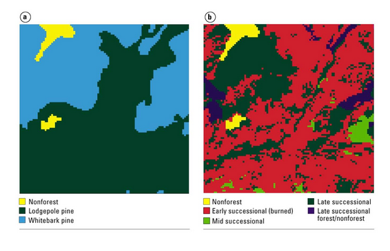
To compare across classification schemes we often have to perform a ‘crosswalk’ in which elements in one classification scheme are mapped to equivalent elements in another scheme. This process can be time consuming and difficult, especially if the two classification schemes are dissimilar.
Next, do the data sets have matching resolution? If not, you will have to generalize the higher resolution data set to the lower resolution of the coarser data set. Generally, the grain of a study area should be two to five times smaller than the size of features of interest (O’Neill et al. 1996).
Below is an example of the effect of changing grain size on a landscape map. Each map shows a 5×5 km section of southwestern Yellowstone National Park, where the grid size is a) 50×50 m b) 100×100 m, and c) 200×200 m.
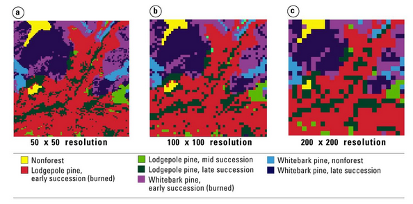
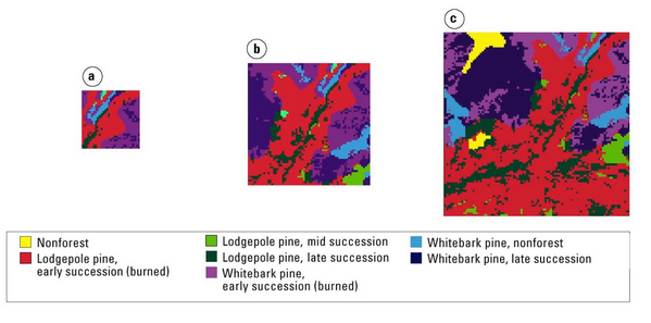
Lastly, do the data sets have matching extent? All spatial data sets should encompass the minimum extent necessary for your analysis. In principle, extent should be two to five times larger than the largest patches (O’Neill et al. 1996).
Below is an example of the effect of changing extent on the landscape map of southwestern Yellowstone National Park. Note that the presence and relative proportions of different land cover types change as the extent of the map changes.
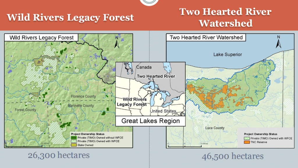
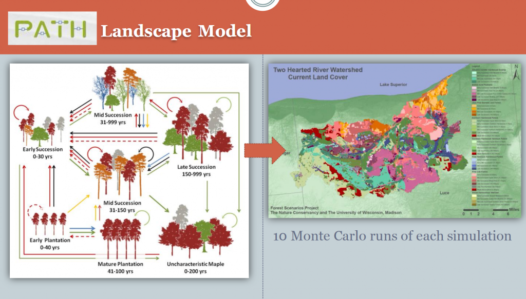
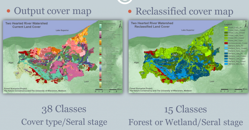
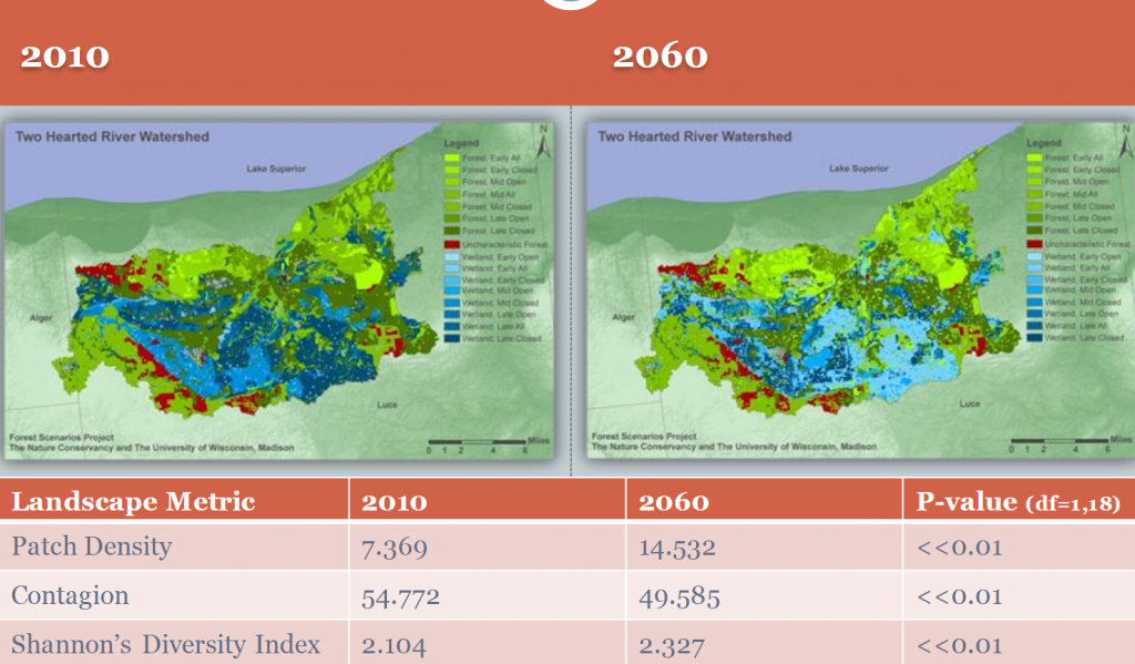
The following set of figures from our Forest Scenarios study illustrates these concepts in a more complex landscape. First, we were working on two different study areas in the Great Lakes region of different extents and management contexts. As a result, we did not attempt to compare between the study areas. The second figure shows the translation from vegetation age and type parameters to a spatial landscape map. Third, because the combined vegetation type and age resulted in 38 classes – too many to make sense of – we condensed those into 15 classes of forest and wetland types and age. This reclass was a sort of ‘cross-walking’. Finally, that allowed us to calculate landscape metrics and reasonably compare between time steps.
2. Preparing for Landscape Metrics
Once our spatial data sets are compatible for comparative landscape assessment, we must make further considerations to prepare for calculating landscape metrics.
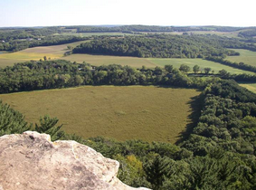
First, we must identify the minimum mappable units that will be quantified. In most landscapes, we start by identifying patches. These may be as small as individual grid cells, but not necessarily.
Most simply defined, a patch is a non-linear surface differing from its surroundings. Often a patch is a cluster or contiguous group of cells (in a raster environment) of the same value or map category.
Yet identifying contiguous cells of the same type can depend on your rules. Different ‘neighbor rules’ can be used to define a contiguous patch.
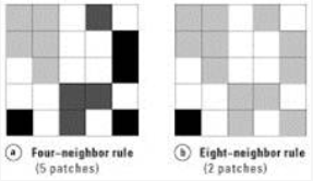
- The four neighbor rule (a) considers any cells of the same class that share a vertical or horizontal border as a single patch.
- The eight neighbor rule (b) considers any cells of the same class that share a vertical, horizontal, or diagonal border as a single patch.
Landscape Metrics
We can quantify pattern first at the landscape level. Landscape metrics can be organized into those that measure:
- landscape composition – the variety of elements in the landscape. What classes are there and how much of each is present?
- landscape configuration – the pattern or spatial arrangements of landscape elements. How are the classes arranged on the landscape?
I like to use cookies to think about how we describe landscapes:

- What are the ingredients in your cookie? Do you like raisins, nuts, oats, or butterscotch chips? That’s composition!
- Are the chocolate chips, raisins, and nuts evenly distributed throughout your cookie, or did they clump up? That’s configuration!
- Are you getting hungry yet?
Metrics for Landscape Composition
The simplest landscape metrics focus on the composition of a landscape, such as which categories are present (raisins, oats, chocolate chips) and how much of the categories there are (more chocolate than raisins), rather than the spatial arrangement of the categories on the landscape.

See the sketches and definitions below to examine metrics designed to assess the composition of a landscape (or what’s in your cookie).
Note: the following definitions and formulas are from Gergel and Turner 2017 and Fragstats (McGarigal et al. 2012).
Patch Richness – the number of different cover classes present on the landscape
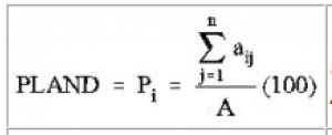
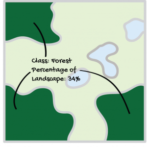
Proportion (PLAND, Pi) – the proportion of the landscape that is occupied by each over class i. This metric is nearly always required, along with other metrics, to describe a landscape.
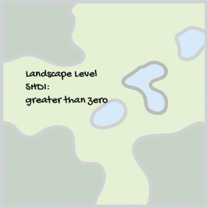
Diversity – refers to how evenly the proportions of cover classes are distributed, also called relative evenness. There are several metrics commonly used to quantify diversity:
- Shannon’s Diversity Index (SHDI) – a popular measure of diversity in community ecology, applied here to landscapes.

Pi =proportion of the landscape occupied by patch type (class) i.
Range: SHDI ≥ 0, without limit
- Shannon’s Evenness Index (SHEI) – expressed such that an even distribution of area among patch types results in maximum evenness. As such, evenness is the complement of dominance.

Pi = proportion of the landscape occupied by patch type (class) i. m = number of patch types (classes) present in the landscape, excluding the landscape border if present
Range: 0 ≦ SHEI ≦ 1
You might be familiar with these diversity indices from plant ecology. Here they are simply applied to measure class diversity rather than plant species.
Dominance – the deviation from maximum possible diversity. Dominance is essentially the inverse of diversity. There are also several possible metrics commonly used to quantify dominance.
- Largest patch index (LPI) – the percentage of total landscape area comprised by the largest patch. As such, it is a simple measure of dominance. LPI can also be calculated for each class individually.

aij = area (m2) of patch ij.
A = total landscape area (m2)
Range: 0 < LPI ≦ 100
Be careful though, similar dominance or diversity values may represent qualitatively very different landscapes.

A variety of landscape metrics are sensitive to the specific spatial arrangement of different cover types in a landscape. In this section, we will consider three components of landscape configuration (or how well the goodies in your cookies were mixed). Notice how the chocolate in these cookies is highly aggregated compared to the chocolate in the chocolate chip cookies.
Note: some formulas will be provided for reference. You don’t need to learn these just yet.
Patch Characteristics
Total number of patches – The total number of patches in the landscape. If total landscape area is held constant, then number of patches conveys the same information as patch density or mean patch size and may be a useful index to interpret.
Patch density (PD) – the total number of patches in the landscape, divided by total landscape area. Patch density has the same basic utility as number of patches as an index, except that it expresses number of patches per unit area, which facilitates comparison among landscapes of varying size. Of course, if total landscape area is held constant, then patch density and number of patches convey the same information.
Edges
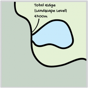
Edge – measures the number or length of edges between cover types per unit area. It is important to make sure that the edges under consideration are ecologically significant. Therefore, it may be more useful to consider the edges between particular cover types than the edge of all cover types at once.
- Total Edge (TE) – total length (m) of edge in landscape involving class type i

eik = total length (m) of edge in landscape involving patch type (class) i; includes landscape boundary and background segments involving patch type i.
- Edge Density (ED) – the sum of the lengths (m) of all edge segments involving the corresponding class type, divided by the total landscape area (m2), multiplied by 10,000 (to convert to hectares).

eik = total length (m) of edge in landscape involving patch type (class) i; includes landscape boundary and background segments involving patch type i.
A = total landscape area (m2)
Aggregation
Adjacency – a measure of the probability that a cell of cover type i is adjacent to a grid cell of a specified cover type.
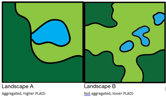
Percent like adjacencies (PLADJ) – measures the degree of aggregation of patch types. PLADJ equals sum of the number of like adjacencies for each patch type, divided by the total number of cell adjacencies in the landscape; multiplied by 100 (to convert to a percentage). In other words, the proportion of cell adjacencies involving the same class.
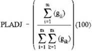
gii = number of like adjacencies (joins) between pixels of patch type (class) i based on the double-count method.
gik = number of adjacencies (joins) between pixels of patch types (classes) i and k based on the double-count method.
Range: 0 ≦ PLADJ ≦ 100
PLADJ equals 0 when the patch types are maximally disaggregated (i.e., every cell is a different patch type) and there are no like adjacencies. PLADJ = 100 when all patch types are maximally aggregated ( i.e., when the landscape consists of single patch and all adjacencies are between the same class).
Thus, a landscape containing larger patches with simple shapes will contain a higher percentage of like adjacencies than a landscape with smaller patches and more complex shapes.
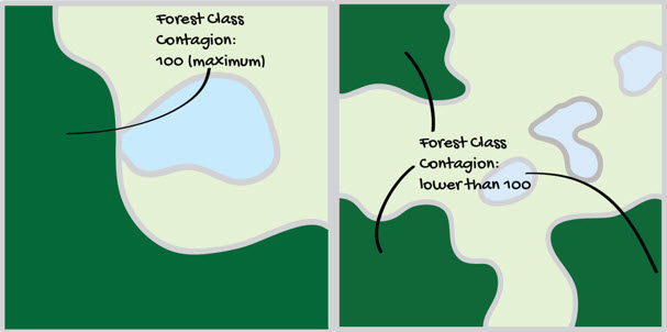
Contagion – differentiates patterns that are ‘clumped’ vs patterns that are ‘dissected,’ sensitive to fine-scale variation.

Pi =proportion of the landscape occupied by patch type (class) i.
gik =number of adjacencies (joins) between pixels of patch types (classes) i and k based on the double-count method.
m =number of patch types (classes) present in the landscape, including the landscape border if present.
Range: 0 < CONTAG ≦ 100
CONTAG approaches 0 when the patch types are maximally disaggregated (i.e., every cell is a different patch type) and interspersed (equal proportions of all pairwise adjacencies). CONTAG = 100 when all patch types are maximally aggregated; i.e., when the landscape consists of single patch.
NOTE: Contagion is inversely related to edge density.
Class Metrics
Once we define patches within the landscape, we can also use metrics to quantify pattern for individual cover classes. Class metrics can describe the size, shape, and aggregation of each cover class separately and are often the basis for landscape metrics that describe the pattern of the landscape as a whole. For each class, we can calculate:
Total class area (CA) – The total area of the landscape occupied by each class.
![]()
aij = area (m2) of patch ij.
Here, CA equals the sum of the areas (m2) of all patches of the corresponding patch type, divided by 10,000 (to convert to hectares). CA approaches 0 as the patch type becomes increasing rare in the landscape.
Number of patches (NP) – The number of patches of each class in the landscape.
Mean patch size (Area_MN) – Average size of the patches of each class.
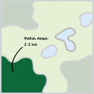
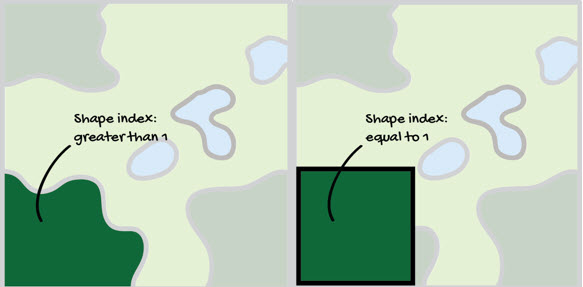
Patch shape index – Measures the area to edge ratio of patches,
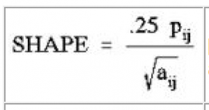
pij = perimeter (m) of patch ij.
aij = area (m2) of patch ij.
Shape index corrects for the size problem of the perimeter-area ratio index, as a result, is the simplest and perhaps most straightforward measure of shape complexity.
Many of the landscape metrics described in the previous section can also be calculated for each class individually.
Most metrics are correlated
Many metrics are correlated, meaning they will capture similar qualities of spatial pattern (Cunningham and Johnson 2011; Wang et al. 2014). Therefore, it is important to select metrics that provide information relevant to the study question or objectives, that are relatively independent (not redundant), and that detect ecologically meaningful properties at the patch, class, or landscape level (Corry and Nassauer 2005; Farr et al. 2017; Kupfer 2012).
This often means choosing multiple metrics that provide information about composition, such as richness of classes or cover types, and configuration, such as edge density and connectivity.
Characteristics of Useful Metrics
- They are chosen to answer a specific question or objective.
- Their measured value is well distributed over the full range of potential values – metrics must vary between time points or landscapes in order to be useful in detecting differences.
- Metrics are relatively independent of one another.
Considerations
- Simple areal metrics are interpretable and easy to calculate (patch area, patch density, edge density, patch size variability, etc.).
- Shape is more difficult to quantify.
- Diversity, richness, and evenness are sensitive to the presence of rare types and hence grain size.
Analysis must recognize the effects of:
- Classification scheme
- Scale and resolution
- Correlation among metrics
Applying Landscape Metrics
Applications of Landscape Pattern Analysis
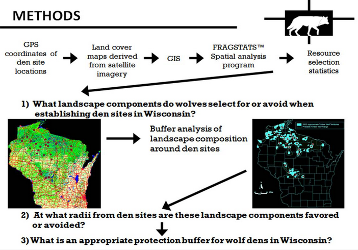
We will explore how landscape pattern analysis can be employed to locate suitable areas for wolf dens in Wisconsin.
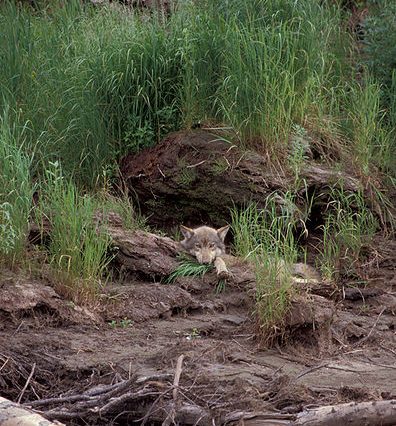
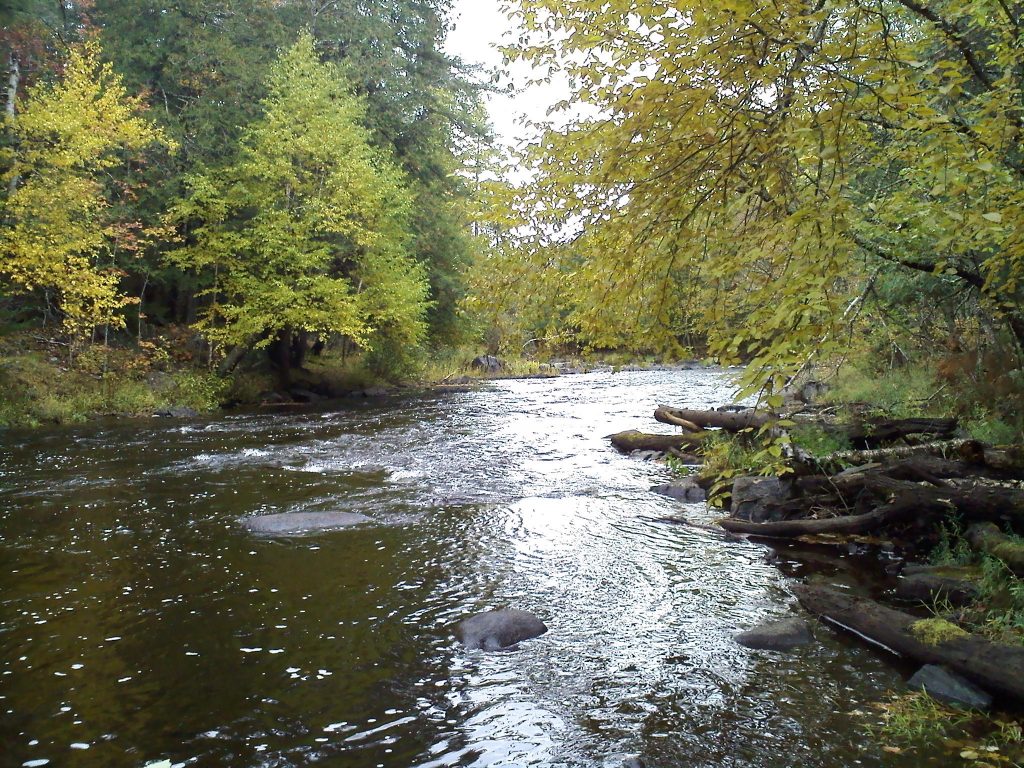
Den site selection is one of the least understood aspects of wolf ecology. Den sites are typically studied qualitatively at a microhabitat scale (i.e. characteristics of physical den and immediate surroundings).
Landscape analysis contributed valuable information to the state of Wisconsin for ensuring a viable wolf population after being relisted as an endangered species in the western Great Lakes region, by answering the following questions:
- What landscape components do wolves select for, or avoid when establishing den sites in Wisconsin?
- At what radii from den sites are these landscape components favored or avoided?
- What is an appropriate protection buffer for wolf dens in Wisconsin?
Methods
Here is an example of an approach used to answer those questions, in part with landscape metrics. In the following pages we will cover each of the key steps in the diagram below.
Land Cover Data
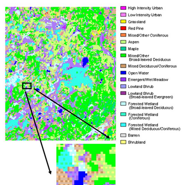
This project chose WISCLAND 1.0 land cover data, the most comprehensive land cover data that was available for the entire state of Wisconsin. WISCLAND shows land cover at 30 m spatial resolution and is based on Landsat Thematic Mapper (TM) satellite data collected in 1992 and 1993.
WISCLAND 2.0, completed in 2016 is a complete update to the previous statewide Wisconsin land cover map.
WISCLAND data was of sufficient spatial resolution for this landscape-scale study and contained a detailed classification of wetland types necessary for understanding the response of wolves to land cover.
Landscape Feature Classes
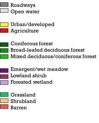
For this study, the WISCLAND land cover data was reclassified according to the classification scheme shown below.
Landscape Analysis
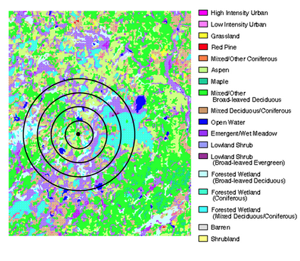
For each known den site, the percent composition of the specified land classifications was measured in circular buffers at 0-500m, 501-1000m, 1001-1500m, and 1501-2000m from the central den site.
Quantifying the amount of each cover type surrounding den sites revealed the landscape feature classes that wolves select for when establishing den sites as well as which features they avoid and at what distance.
The composition surrounding known den sites was compared to the total availability of each coverage type within each wolf pack’s known annual territory to locate other areas of similar composition. These areas of similar composition are possible locations of new denning sites.
Together this information could inform conservation and land use planning in light of wolf habitat needs.
Landscape Metrics
These are the metrics that were chosen to quantify the landscape surrounding den sites:
Landscape Composition
- Proportion (PLAND) – of each cover type present
- Diversity – how evenly the proportions of cover types are distributed
Spatial Configuration
- Probabilities of Adjacency (PLADJ) – probability that a grid cell of cover type i is adjacent to a grid cover type j
- Patch Area and Perimeter
The project used FRAGSTATS, a GIS-based landscape structure and spatial analysis program (McGarigal and Marks 1995), to calculate habitat composition metrics on a landscape scale.
A Note on Significant Digits
As you learn to work with programs like FRAGSTATS, be thoughtful about the numerical results that you report. Significant digits are still important.
The number of decimal places in a number is determined by the precision of the measurement. Therefore, the results of any mathematical manipulations of measurements can only be reported with the same number of significant figures as the least precise of the numbers being used.
Example:
5.67 (two decimal places)
1.1 (one decimal place)
+0.9378 (four decimal place)
7.7 (one decimal place)
The Two Greatest Sins Regarding Significant Digits
- Writing more digits in an answer (intermediate or final) than justified by the number of significant digits in the data.
- Rounding-off, say, to two digits in an intermediate answer, and then writing three digits in the final answer.
For more help with significant digits, watch this Khan Academy video on Significant Digits.
References:
- Landscape metric illustrations by G.Martius, CC BY-NC-SA 4.0
- Corry, R. C., & Nassauer, J. I. (2005). Limitations of using landscape pattern indices to evaluate the ecological consequences of alternative plans and designs. Landscape and urban planning, 72(4), 265-280.
- Cunningham, M. A., & Johnson, D. H. (2011). Seeking parsimony in landscape metrics. The Journal of wildlife management, 75(3), 692-701.
- Farr, Cooper M. ; Pejchar, Liba ; Reed, Sarah E. 2017. Subdivision design and stewardship affect bird and mammal use of conservation developments. Ecological Applications, Vol.27(4), pp.1236-1252
- Gergel and Turner, 2017, 2nd edition, chapter 4.
- Kupfer, J. A. (2012). Landscape ecology and biogeography: rethinking landscape metrics in a post-FRAGSTATS landscape. Progress in Physical Geography, 36(3) 400-420.
- McGarigal, K., SA Cushman, and E Ene. 2012. FRAGSTATS v4: Spatial Pattern Analysis Program for Categorical and Continuous Maps. Computer software program produced by the authors at the University of Massachusetts, Amherst. Available at the following web site: http://www.umass.edu/landeco/research/fragstats/fragstats.html
- McGarigal K. and BJ Marks. 1995. FRAGSTATS. Spatial analysis program for quantifying landscape structure. USDA Forest Servicee General Technical Report PNW-GTR-351.
- O’Neill, RV, CT Hunsaker, SP Timmins, BL Jackson, KB Jones, KH Riiters, JD Wickham. 1996. Scale problems in reporting landscape pattern at the regional scale. Landscape Ecology 11:169-180.
- Price, J., Silbernagel, J. Nixon, K., Swearingen, A., Swaty, R. and N.Miller. 2015. Collaborative scenario modeling reveals potential advantages of blending strategies to achieve conservation goals in a working forest landscape. Landscape Ecology doi:10.1007/s10980-015-0321-2
Turner and Gardner, 2015, 2nd edition, chapter 4. - White, Annie. 20xx. MS Thesis, University of Wisconsin-Madison. – gathering specific title & year
- Wang, X., Blanchet, F. G., & Koper, N. (2014). Measuring habitat fragmentation: an evaluation of landscape pattern metrics. Methods in Ecology and Evolution, 5(7), 634-646.
