1. Introduction

In this appendix we will learn that there are different ways of implementing any particular model, and we will discuss how to choose the most appropriate implementation for a given purpose. To this end, we consider three different algorithms agents may use as a decision rule which lead to the same (probabilistic) output, i.e., they lead to the same conditional probabilities that a reviser using strategy switches to strategy . Therefore, these three algorithms lead to exactly the same dynamics. Nonetheless, the three algorithms differ in efficiency, code readability, and on how realistic the story behind them may sound.

2. Three possible stories behind the same behavior

In this section we present three different algorithms agents may use as a decision rule which lead to the same conditional probabilities , where is the fraction of -strategists and is the average payoff of -strategists.

2.1. Vose’s alias method

The following decision rule uses NetLogo primitive rnd:weighted-one-of, which returns one agent selected stochastically. The probability of each agent being picked is proportional to her payoff. Once the agent is selected, the reviser copies her strategy.

to Vose-alias-imitate-positive-proportional-rule
  ;; assumes that all payoffs are non-negative
  let chosen-player rnd:weighted-one-of players [payoff]
  set next-strategy [strategy] of chosen-player
end

Primitive rnd:weighted-one-of in NetLogo 6.4.0 uses Keith Schwarz’s (2011) implementation of Vose’s (1991) alias method. This algorithm is very efficient (especially when several draws are required), but we would find it hard to sell as an actual procedure that human agents may use to select a strategy.

2.2. Roulette wheel

The following decision rule implements the so-called “roulette wheel selection algorithm” to select one agent with probability proportional to payoffs. Let be the number of agents and let be player ‘s payoff. The algorithm starts by assigning one line segment of length to each agent . These segments are then placed consecutively to build a larger segment of length equal to the sum of all players’ payoffs (Figure 1).

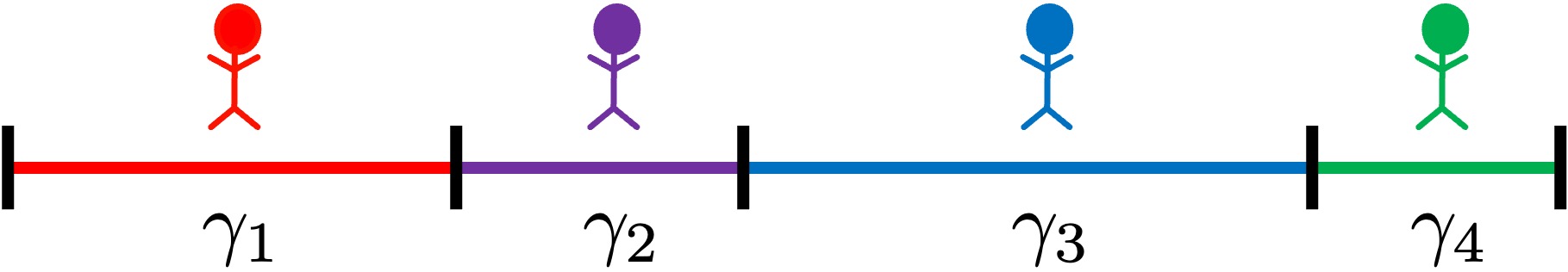
We then obtain a random number between 0 and (i.e. a random location in the big segment), and we select the agent who owns that part of the big segment. Once the agent is selected, the reviser copies her strategy.^[1] The following decision rule is an inefficient but quite readable implementation of this algorithm in NetLogo.

to roulette-wheel-imitate-positive-proportional-rule
  ;; assumes that all payoffs are non-negative

  ;; returns the strategy of one agent selected
  ;; with probability proportional to payoffs,
  ;; using an inneficient implementation of 
  ;; the roulette wheel algorithm

  let list-of-agents sort players
  let list-of-payoffs map [a -> [payoff] of a] list-of-agents

  if (sum list-of-payoffs = 0) [
    ;; applies when all players have payoff = 0
    set list-of-payoffs n-values n-of-players [1]
  ]
  
  let cumulative-payoffs [0]
  foreach list-of-payoffs [p ->
    set cumulative-payoffs lput (p + last cumulative-payoffs) 
                                 cumulative-payoffs
  ]
    ;; cumulative-payoffs is (n-of-players + 1) items long,
    ;; its first value is 0 and its last value is the sum of all payoffs.
    ;; You can also use reduce instead of foreach for a 
    ;; more efficient but less readable implementation
 
  let rd-number random-float (last cumulative-payoffs)
    ;; take a random number between 0 and 
    ;; the sum of all payoffs

  let index length filter [p -> rd-number >= p] 
                   (butfirst cumulative-payoffs)
    ;; see in which player's segment the random number is located.
    ;; The efficiency of this process can be greatly improved
    ;; by using e.g. binary search

  let chosen-player (item index list-of-agents)
  set next-strategy [strategy] of chosen-player
end

2.3. Repeated sampling

In this section we provide an implementation of an algorithm that Sandholm (2010a, example 5.4.5) calls “repeated sampling”.^[2] The algorithm works as follows:

1. The reviser sets a random aspiration level in the interval , where is the maximum payoff in the population of agents.^[3]
2. The reviser selects one agent at random. Let denote this selected agent and let be her payoff.
3. If , i.e., if the observed agent’s payoff is greater than or equal to the reviser’s aspiration, then the reviser copies the observed agent’s strategy. Otherwise the reviser goes back to step 1.

Below you can find an implementation of this algorithm in Netlogo.

to repeated-sampling-imitate-positive-proportional-rule
  ;; assumes that all payoffs are non-negative
  loop [
    let my-random-aspiration random-float max-payoff
    let one-at-random one-of players
    if [payoff] of one-at-random >= my-random-aspiration [
      set next-strategy [strategy] of one-at-random
      stop
    ]
  ]
end

Note that, in contrast with the two previous algorithms, in this case the reviser will not generally use the payoffs of every player. The algorithm does require that the reviser has access to all the payoffs and, in the worst-case scenario, the algorithm will use them; but, in general, the reviser will most likely use just a few of those payoffs.

3. Which algorithm should we use?

The three decision rules above provide exactly the same conditional probabilities . This means that if we only observed the actions of the agents, it would be impossible to tell which of the three algorithms the agents are using. The three decision rules lead to exactly the same dynamics. For this reason, we could say that they are:

• three different micro-foundations for the same model,
• three different decision rules that give the same output, or
• in the context of population games, three different implementations of the same revision protocol (Sandholm, 2010a).

Personally, if we had to motivate the decision rule, we would probably use the story behind repeated sampling. This decision rule seems the most natural of the three as a decision-making algorithm and, in general, it requires less information than the other two.

If we wanted to prioritize code readability, we would choose NetLogo primitive rnd:weighted-one-of, as we did in the implementation of procedure to imitative-positive-proportional-m-rule in chapters III-4 and IV-4.

And finally, to run several simulations, knowing that the three decision rules lead to exactly the same dynamics, we would choose the most efficient one. This would imply ruling out our naive implementation of the “roulette wheel selection algorithm”. The relative efficiency of the other two decision rules depends on various factors such as the number of agents, the distribution of payoffs, and the number of times we want to execute the algorithm for a fixed distribution of payoffs.^[4] In our models, it turns out that repeated sampling is often the most efficient decision rule too. For details on the efficiency and the intuition behind these three algorithms (and some others), see Keith Schwarz’s (2011) excellent web page “Darts, Dice, and Coins: Sampling from a Discrete Distribution“.