Part II. Our first agent-based evolutionary model
II-5. Analysis of these models
1. Two complementary approaches
Agent-based models are usually analyzed using computer simulation and/or mathematical analysis.
- The computer simulation approach consists in running many simulations –i.e. sampling the model many times– and then, with the data thus obtained, trying to infer general patterns and properties of the model.
- Mathematical approaches do not look at individual simulation runs, but instead analyze the rules that define the model directly, and try to derive their logical implications. Mathematical approaches use deductive reasoning only, so their conclusions follow with logical necessity from the assumptions embedded in the model (and in the mathematics employed).
These two approaches are complementary, in that they can provide fundamentally different insights on the same model. Furthermore, there are synergies to be exploited by using the two approaches together (see e.g. Izquierdo et al. (2013, 2019), Seri (2016), Hilbe and Traulsen (2016), García and van Veelen (2016, 2018) and Hindersin et al. (2019)).
Here we provide several references to material that is helpful to analyze the agent-based models we have developed in this Part II of the book, and illustrate its usefulness with a few examples. Section 2 below deals with the computer simulation approach, while section 3 addresses the mathematical analysis approach.
2. Computer simulation approach
The task of running many simulation runs –with the same or different combinations of parameter values– is greatly facilitated by a tool named BehaviorSpace, which is included within NetLogo and is very well documented at NetLogo website. Here we provide an illustration of how to use it.
Consider a coordination game defined by payoffs [[1 0][0 2]], played by 1000 agents who simultaneously revise their strategies with probability 0.01 in every tick, following the imitate if better rule without noise. This is the model implemented in the previous chapter, and it can be downloaded here (nxn-imitate-if-better-noise-efficient.nlogo). This model is stochastic and we wish to study how it usually behaves, departing from a situation where both strategies are equally represented. To that end, we could run several simulation runs (say 1000) and plot the average fraction of 1-strategists in every tick, together with the minimum and the maximum values observed across runs in every tick. An illustration of this type of graph is shown in figure 1. Recall that strategies are labeled 0 and 1, so strategy 1 is the one that can get a payoff of 2.
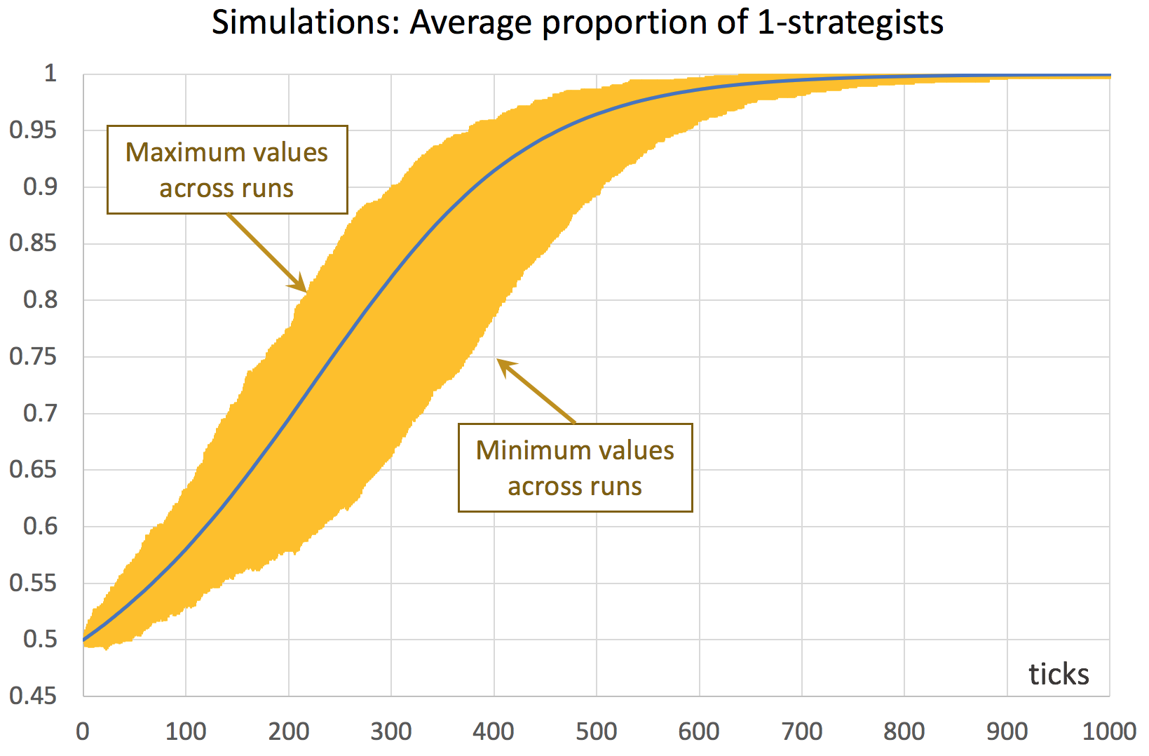
To set up the computational experiment that will produce the data required to draw figure 1, we just have to go to Tools (in the upper menu of NetLogo) and then click on BehaviorSpace. The new experiment can be set up as shown in figure 2.
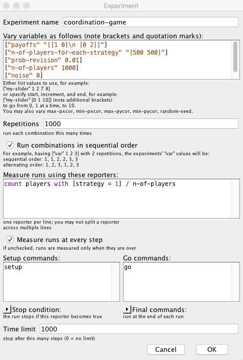
In this particular experiment, we are not changing the value of any parameter, but doing so is straightforward. For instance, if we wanted to run simulations with different values of prob-revision –say 0.01, 0.05 and 0.1–, we would just write:
[ "prob-revision" 0.01 0.05 0.1 ]
If, in addition, we would like to explore the values of noise 0, 0.01, 0.02 … 0.1, we could use the syntax for loops, [start increment end], as follows:
[ "noise" [0 0.01 0.1] ] ;; note the additional brackets
If we made the two changes described above, then the new computational experiment would comprise 33000 runs, since NetLogo would run 1000 simulations for each combination of parameter values (i.e. 3 × 11).
The original experiment shown in figure 2, which consists of 1000 simulation runs only, takes a couple of minutes to run. Once it is completed, we obtain a .csv file with all the requested data, i.e. the fraction of 1-strategists in every tick for each of the 1000 simulation runs – a total of 1001000 data points. Then, with the help of a pivot table (within e.g. an Excel spreadsheet), it is easy to plot the graph shown in figure 1. A similar graph that can be easily plotted is one that shows the standard error of the average computed in every tick (see figure 3).[1]

3. Mathematical analysis approach. Markov chains
From a mathematical point of view, agent-based models can be usefully seen as time-homogeneous Markov chains (see Gintis (2013) and Izquierdo et al. (2009) for several examples). Doing so can make evident many features of the model that are not apparent before formalizing the model as a Markov chain. Thus, our first recommendation is to learn the basics of this theory. Karr (1990), Kulkarni (1995, chapters 2-4), Norris (1997), Kulkarni (1999, chapter 5), and Janssen and Manca (2006, chapter 3) are all excellent introductions to the topic.
All the models developed in this Part II can be seen as time-homogeneous Markov chains on the finite space of possible strategy distributions. This means that the number of agents that are using each possible strategy is all the information we need to know about the present –and the past– of the stochastic process in order to be able to –probabilistically– predict its future as accurately as it is possible. Thus, the number of possible states in these models is ![]() , where
, where ![]() is the number of agents and
is the number of agents and ![]() the number of strategies.[2]
the number of strategies.[2]
In some simple cases, a full Markov analysis can be conducted by deriving the transition probabilities of the Markov chain and operating directly with them. Section 3.1 illustrates how this type of analysis can be undertaken on models with 2 strategies where agents revise their strategies sequentially.
However, in many other models a full Markov analysis is unfeasible because the exact formulas can lead to very cumbersome expressions, or may even be too complex to evaluate. This is often the case if the number of states is large.[3] In such situations, one can still take advantage of powerful approximation results, which we introduce in section 3.2.
3.1. Markov analysis of 2-strategy evolutionary processes where agents switch strategies sequentially
In this section we study 2-strategy evolutionary processes where agents switch strategies sequentially. For simplicity, we will asume that there is one revision per tick, but several revisions could take place in the same tick as long as they occurred sequentially. These processes can be formalized as birth-death chains, a special type of Markov chains for which various analytical results can be derived.
Note that, in the model implemented in the previous chapter (and simulated in section 2 above), agents do not revise their strategies sequentially, but simultaneously within the tick. The difference between these two updating schemes are small for low probabilities of revision, so the formal analysis presented here will be useful to analyze the computer model as long prob-revision is not too high.
3.1.1. Markov chain formulation
Consider a population of ![]() agents who repeatedly play a symmetric 2-player 2-strategy game. The two possible strategies are labeled 0 and 1. In every tick, one random agent is given the opportunity to revise his strategy, and he does so according to a certain decision rule (such as the imitate if better rule, the imitative pairwise-difference rule or the best experienced payoff rule).
agents who repeatedly play a symmetric 2-player 2-strategy game. The two possible strategies are labeled 0 and 1. In every tick, one random agent is given the opportunity to revise his strategy, and he does so according to a certain decision rule (such as the imitate if better rule, the imitative pairwise-difference rule or the best experienced payoff rule).
Let ![]() be the proportion of the population using strategy 1 at tick
be the proportion of the population using strategy 1 at tick ![]() . The evolutionary process described above induces a Markov chain
. The evolutionary process described above induces a Markov chain ![]() on the state space
on the state space ![]() . We do not have to keep track of the proportion of agents using strategy 0 because there are only two strategies, so the two proportions must add up to one. Since there is only one revision per tick, note that there are only three possible transitions: one implies increasing
. We do not have to keep track of the proportion of agents using strategy 0 because there are only two strategies, so the two proportions must add up to one. Since there is only one revision per tick, note that there are only three possible transitions: one implies increasing ![]() by
by ![]() , another one implies decreasing
, another one implies decreasing ![]() by
by ![]() , and the other one leaves the state unchanged. Let us denote the transition probabilities as follows:
, and the other one leaves the state unchanged. Let us denote the transition probabilities as follows:
![]()
![]()
Thus, the probability of staying at the same state after one tick is:
![]()
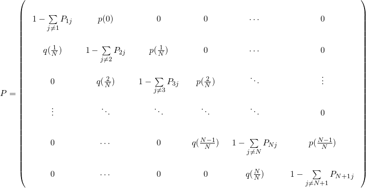
This Markov chain has two important properties: the state space ![]() is endowed with a linear order and all transitions move the state one step to the left, one step to the right, or leave the state unchanged. These two properties imply that the Markov chain is a birth-death chain. Figure 4 below shows the transition diagram of this birth-death chain, ignoring the self-loops.
is endowed with a linear order and all transitions move the state one step to the left, one step to the right, or leave the state unchanged. These two properties imply that the Markov chain is a birth-death chain. Figure 4 below shows the transition diagram of this birth-death chain, ignoring the self-loops.

The transition matrix ![]() of a Markov chain gives us the probability of going from one state to another. In our case, the elements
of a Markov chain gives us the probability of going from one state to another. In our case, the elements ![]() of the transition matrix are:
of the transition matrix are:
In our evolutionary process, the transition probabilities ![]() and
and ![]() are determined by the decision rule that agents use. Let us see how this works with a specific example. Consider the coordination game defined by payoffs [[1 0][0 2]], played by agents who sequentially revise their strategies according to the imitate if better rule (without noise). This is very similar to the model we have simulated in section 2 above. The only difference is that now we are assuming revisions take place sequentially, while in the model simulated in section 2 agents revise their strategies simultaneously within the tick (with probability 0.01). Assuming that the fraction of agents that revise their strategies simultaneously is low (in this case, about 1%), the difference between the formal model and the computer model will be small.[4]
are determined by the decision rule that agents use. Let us see how this works with a specific example. Consider the coordination game defined by payoffs [[1 0][0 2]], played by agents who sequentially revise their strategies according to the imitate if better rule (without noise). This is very similar to the model we have simulated in section 2 above. The only difference is that now we are assuming revisions take place sequentially, while in the model simulated in section 2 agents revise their strategies simultaneously within the tick (with probability 0.01). Assuming that the fraction of agents that revise their strategies simultaneously is low (in this case, about 1%), the difference between the formal model and the computer model will be small.[4]
Let us derive ![]() . Note that the state increases by
. Note that the state increases by ![]() if and only if the revising agent is using strategy 0 and he switches to strategy 1. In the game with payoffs [[1 0][0 2]], this happens if and only if the following conditions are satisfied:
if and only if the revising agent is using strategy 0 and he switches to strategy 1. In the game with payoffs [[1 0][0 2]], this happens if and only if the following conditions are satisfied:
- the agent who is randomly drawn to revise his strategy is playing strategy 0 (an event which happens with probability
 ),
), - the agent that is observed by the revising agent is playing strategy 1 (an event which happens with probability
 ; note that there are
  agents using strategy 1 and the revising agent observes another agent, thus the divisor
  ), and
 - the observed agent’s payoff is 2, i.e. the observed agent –who is playing strategy 1– played with an agent who was also playing strategy 1 (an event which happens with probability
 ; note that the observed agent plays with another agent who is also playing strategy 1).
Therefore:
![]()
Note that, in this case, the payoff obtained by the revising agent is irrelevant.
We can derive ![]() in a similar fashion. Do you want to give it a try before reading the solution?
in a similar fashion. Do you want to give it a try before reading the solution?
Computation of 
Note that the state decreases by ![]() if and only if the revising agent is using strategy 1 and he switches to strategy 0. In the game with payoffs [[1 0][0 2]], this happens if and only if the following conditions are satisfied:
if and only if the revising agent is using strategy 1 and he switches to strategy 0. In the game with payoffs [[1 0][0 2]], this happens if and only if the following conditions are satisfied:
- the agent who is randomly drawn to revise his strategy is playing strategy 1 (an event which happens with probability
 ),
), - the agent that is observed by the revising agent is playing strategy 0 (an event which happens with probability
 ; note that there are
  0-strategists and the revising agent observes another agent, thus the divisor
  ),
), - the revising agent’s payoff is 0, i.e. the revising agent played with an agent who was playing strategy 0 (an event which happens with probability
 ; note that the revising agent plays with another agent, thus the divisor
  ).
). - the observed agent’s payoff is 1, i.e. the observed agent, who is playing strategy 0, played with an agent who was also playing strategy 0 (an event which happens with probability
 ; note that the observed agent plays with another agent who is also playing strategy 0).
Therefore:
![]()
With the formulas of ![]() and
and ![]() in place, we can write the transition matrix of this model for any given
in place, we can write the transition matrix of this model for any given ![]() . As an example, this is the transition matrix
. As an example, this is the transition matrix ![]() for
for ![]() :
:
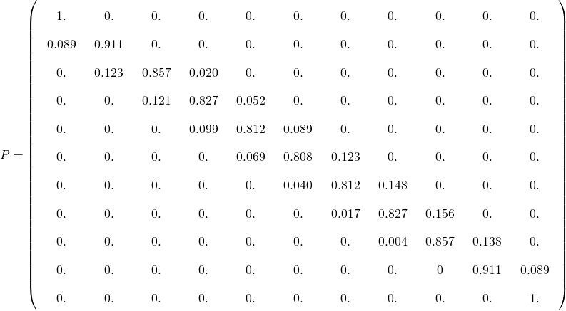
And here’s a little Mathematica® script that can be used to generate the transition matrix for any ![]() :
:
n = 10;
p[x_] := (1 - x) (x n/(n - 1)) ((x n - 1)/(n - 1))
q[x_] := x (((1 - x)n)/(n - 1))^2 ((1 - x)n - 1)/(n - 1)

P = SparseArray[{
    {i_, i_} -> (1 - p[(i - 1)/n] - q[(i - 1)/n]),
    {i_, j_} /; i == j - 1 -> p[(i - 1)/n],
    {i_, j_} /; i == j + 1 -> q[(i - 1)/n]
    }, {n + 1, n + 1}];

MatrixForm[P]
3.1.2. Transient dynamics
In this section, we use the transition matrix ![]() we have just derived to compute the transient dynamics of our two-strategy evolutionary process, i.e. the probability distribution of
we have just derived to compute the transient dynamics of our two-strategy evolutionary process, i.e. the probability distribution of ![]() at a certain
at a certain ![]() . Naturally, this distribution generally depends on initial conditions.
. Naturally, this distribution generally depends on initial conditions.
To be concrete, imagine we set some initial conditions, which we express as a (row) vector ![]() containing the initial probability distribution over the
containing the initial probability distribution over the ![]() states of the system at tick
states of the system at tick ![]() , i.e.
, i.e. ![]() , where
, where ![]() . If initial conditions are certain, i.e. if
. If initial conditions are certain, i.e. if ![]() , then all elements of
, then all elements of ![]() are 0 except for
are 0 except for ![]() , which would be equal to 1.
, which would be equal to 1.
Our goal is to compute the vector ![]() , which contains the probability of finding the process in each of the possible
, which contains the probability of finding the process in each of the possible ![]() states at tick
states at tick ![]() (i.e. after
(i.e. after ![]() revisions), having started at initial conditions
revisions), having started at initial conditions ![]() . This
. This ![]() is a row vector representing the probability mass function of
is a row vector representing the probability mass function of ![]() .
.
To compute ![]() , it is important to note that the
, it is important to note that the ![]() -step transition probabilities
-step transition probabilities ![]() are given by the entries of the
are given by the entries of the ![]() th power of the transition matrix, i.e.:
th power of the transition matrix, i.e.:
![]()
Thus, we can easily compute the transient distribution ![]() simply by multiplying the initial conditions
simply by multiplying the initial conditions ![]() by the
by the ![]() th power of the transition matrix
th power of the transition matrix ![]() :
:
![]()
As an example, consider the evolutionary process we formalized as a Markov chain in the previous section, with ![]() imitate if better agents playing the coordination game [[1 0][0 2]]. Let us start at initial state
imitate if better agents playing the coordination game [[1 0][0 2]]. Let us start at initial state ![]() , i.e.
, i.e. ![]() , where the solitary 1 lies exactly at the middle of the vector
, where the solitary 1 lies exactly at the middle of the vector ![]() (i.e. at position
(i.e. at position ![]() ). Figure 5 shows the distributions
). Figure 5 shows the distributions ![]() and
and ![]() .
.
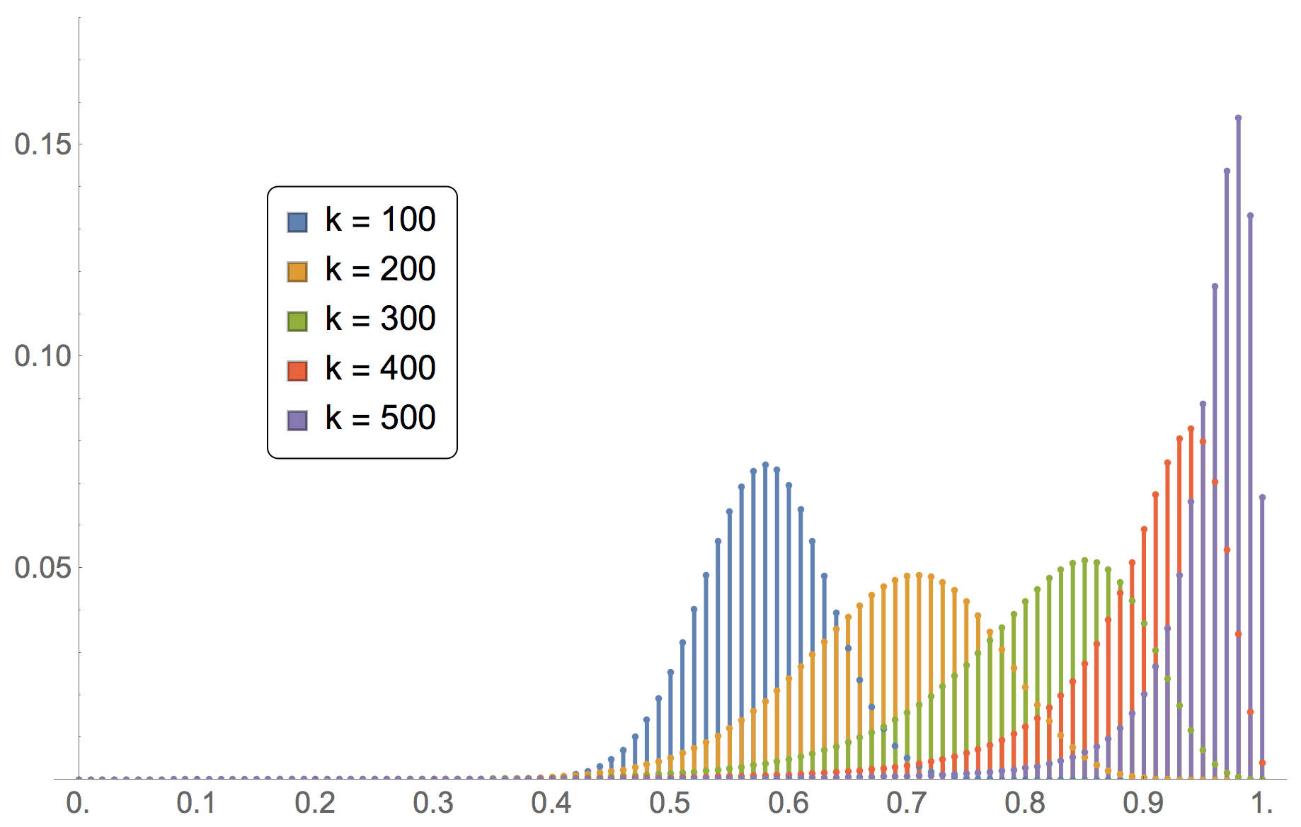
 at different ticks. Number of agents
  . Initial conditions
To produce figure 5, we have computed the transition matrix with the previous Mathematica® script (having previously set the number of agents to 100) and then we have run the following two lines:
a0 = UnitVector[n + 1, 1 + n/2];
ListPlot[Table[a0.MatrixPower[N@P, i], {i, 100, 500, 100}], PlotRange -> All]
Looking at the probability distribution of ![]() , it is clear that, after 500 revisions, the evolutionary process is very likely to be at a state where most of the population is using strategy 1. There is even a substantial probability (~6.66%) that the process will have reached the absorbing state where everyone in the population is using strategy 1. Note, however, that all the probability distributions shown in figure 5 have full support, i.e. the probability of reaching the absorbing state where no one uses strategy 1 after 100, 200, 300, 400 or 500 is very small, but strictly positive. As a matter of fact, it is not difficult to see that, given that
, it is clear that, after 500 revisions, the evolutionary process is very likely to be at a state where most of the population is using strategy 1. There is even a substantial probability (~6.66%) that the process will have reached the absorbing state where everyone in the population is using strategy 1. Note, however, that all the probability distributions shown in figure 5 have full support, i.e. the probability of reaching the absorbing state where no one uses strategy 1 after 100, 200, 300, 400 or 500 is very small, but strictly positive. As a matter of fact, it is not difficult to see that, given that ![]() and
and ![]() (i.e. initially there are 50 agents using strategy 1),
(i.e. initially there are 50 agents using strategy 1), ![]() for any
for any ![]() .
.
Finally, to illustrate the sensitivity of transient dynamics to initial conditions, we replicate the computations shown in figure 5, but with initial conditions ![]() (figure 6) and
(figure 6) and ![]() (figure 7).
(figure 7).
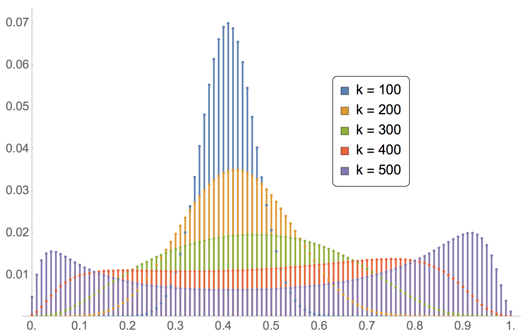
 at different ticks. Number of agents
  . Initial conditions
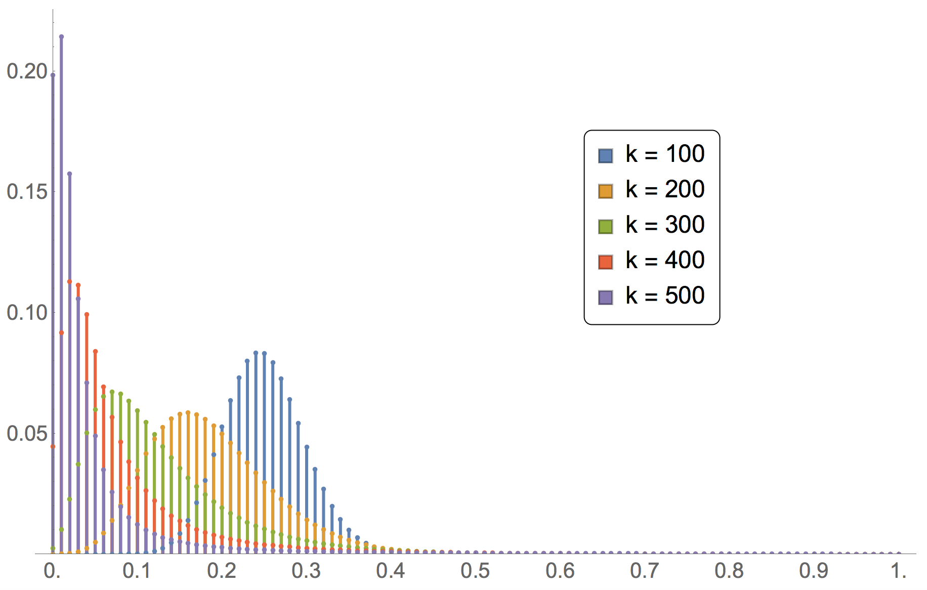
 at different ticks. Number of agents
  . Initial conditions
Besides the probability distribution of ![]() at a certain
at a certain ![]() , we can analyze many other interesting properties of a Markov chain, such as the expected hitting time (or first passage time) of a certain state
, we can analyze many other interesting properties of a Markov chain, such as the expected hitting time (or first passage time) of a certain state ![]() , which is the expected time at which the process first reaches state
, which is the expected time at which the process first reaches state ![]() . For general Markov chains, this type of results can be found in any of the references mentioned at the beginning of section 3. For birth-death chains specifically, Sandholm (2010a, section 11.A.3) provides simple formulas to compute expected hitting times and hitting probabilities (i.e. the probability that the birth-death chain reaches state
. For general Markov chains, this type of results can be found in any of the references mentioned at the beginning of section 3. For birth-death chains specifically, Sandholm (2010a, section 11.A.3) provides simple formulas to compute expected hitting times and hitting probabilities (i.e. the probability that the birth-death chain reaches state ![]() before state
before state ![]() ).
).
3.1.3. Infinite-horizon behavior
In this section we wish to study the infinite-horizon behavior of our evolutionary process, i.e. the distribution of ![]() when the number of ticks
when the number of ticks ![]() tends to infinity. This behavior generally depends on initial conditions, but we focus here on a specific type of Markov chain (irreducible and aperiodic) whose limiting behavior does not depend on initial conditions. To understand the concepts of irreducibility and aperiodicity, we recommend you read any of the references on Markov chains provided at the beginning of section 3. Here we just provide sufficient conditions that guarantee that a (time-homogeneous) Markov chain is irreducible and aperiodic:
tends to infinity. This behavior generally depends on initial conditions, but we focus here on a specific type of Markov chain (irreducible and aperiodic) whose limiting behavior does not depend on initial conditions. To understand the concepts of irreducibility and aperiodicity, we recommend you read any of the references on Markov chains provided at the beginning of section 3. Here we just provide sufficient conditions that guarantee that a (time-homogeneous) Markov chain is irreducible and aperiodic:
Sufficient conditions for irreducibility and aperiodicity of time-homogeneous Markov chains
- If it is possible to go from any state to any other state in one single step (
 for all
  ) and there are more than 2 states, then the Markov chain is irreducible and aperiodic.
 - If it is possible to go from any state to any other state in a finite number of steps, and there is at least one state in which the system may stay for two consecutive steps (
 for some
  ), then the Markov chain is irreducible and aperiodic.
 - If there exists a positive integer
 such that
  for all
  and
and  , then the Markov chain is irreducible and aperiodic.
If one sees the transition diagram of a Markov chain (see e.g. Figure 4 above) as a directed graph (or network), the conditions above can be rewritten as:
- The network contains more than two nodes and there is a directed link from every node to every other node.
- The network is strongly connected and there is at least one loop.
- There exists a positive integer
 such that there is at least one walk of length
from any node to every node (including itself).
The 2-strategy evolutionary process we are studying in this section is not necessarily irreducible if there is no noise. For instance, the coordination game played by imitate-if-better agents analyzed in section 3.1.2 is not irreducible. That model will eventually reach one of the two absorbing states where all the agents are using the same strategy, and stay in that state forever. The probability of ending up in one or the other absorbing state depends on initial conditions (see Figure 8).[5]

 , in the coordination game [[1 0][0 2]] played by
  imitate-if-better agents
However, if we add noise in the agents’ decision rule –so there is always the possibility that revising agents choose any strategy–, then it is easy to see that the second sufficient condition for irreducibility and aperiodicity above is fulfilled.[6]
Generally, in irreducible and aperiodic Markov chains ![]() with state space
with state space ![]() (henceforth IAMCs), the probability mass function of
(henceforth IAMCs), the probability mass function of ![]() approaches a limit as
approaches a limit as ![]() tends to infinity. This limit is called the limiting distribution, and is denoted here by
tends to infinity. This limit is called the limiting distribution, and is denoted here by ![]() , a vector with components
, a vector with components ![]() which denote the probability of finding the system in state
which denote the probability of finding the system in state ![]() in the long run. Formally, in IAMCs the following limit exists and is unique (i.e. independent of initial conditions):
in the long run. Formally, in IAMCs the following limit exists and is unique (i.e. independent of initial conditions):
![]()
Thus, in IAMCs the probability of finding the system in each of its states in the long run is strictly positive and independent of initial conditions. Importantly, in IAMCs the limiting distribution ![]() coincides with the occupancy distribution
coincides with the occupancy distribution ![]() , which is the long-run fraction of the time that the IAMC spends in each state.[7] This means that we can estimate the limiting distribution
, which is the long-run fraction of the time that the IAMC spends in each state.[7] This means that we can estimate the limiting distribution ![]() of a IAMC using the computer simulation approach by running just one simulation for long enough (which enables us to estimate
of a IAMC using the computer simulation approach by running just one simulation for long enough (which enables us to estimate ![]() ).
).
In any IAMC, the limiting distribution ![]() can be computed as the left eigenvector of the transition matrix
can be computed as the left eigenvector of the transition matrix ![]() corresponding to eigenvalue 1.[8] Note, however, that computing eigenvectors is computationally demanding when the state space is large. Fortunately, for irreducible and aperiodic birth-death chains (such as our 2-strategy evolutionary process with noise), there is an analytic formula for the limiting distribution that is easy to evaluate:[9]
corresponding to eigenvalue 1.[8] Note, however, that computing eigenvectors is computationally demanding when the state space is large. Fortunately, for irreducible and aperiodic birth-death chains (such as our 2-strategy evolutionary process with noise), there is an analytic formula for the limiting distribution that is easy to evaluate:[9]
![]()
where the value of ![]() is derived by imposing that the elements of
is derived by imposing that the elements of ![]() must add up to 1. This formula can be easily implemented in Mathematica®:
must add up to 1. This formula can be easily implemented in Mathematica®:
μ = Normalize[FoldList[Times, 1, Table[p[(j-1)/n]/q[j/n],{j, n}]], Total]
Note that the formula above is only valid for irreducible and aperiodic birth-death chains. An example of such a chain would be the model where a number of imitate if better agents are playing the coordination game [[1 0][0 2]] with noise. Thus, for this model we can easily analyze the impact of noise on the limiting distribution. Figure 9 illustrates this dependency.
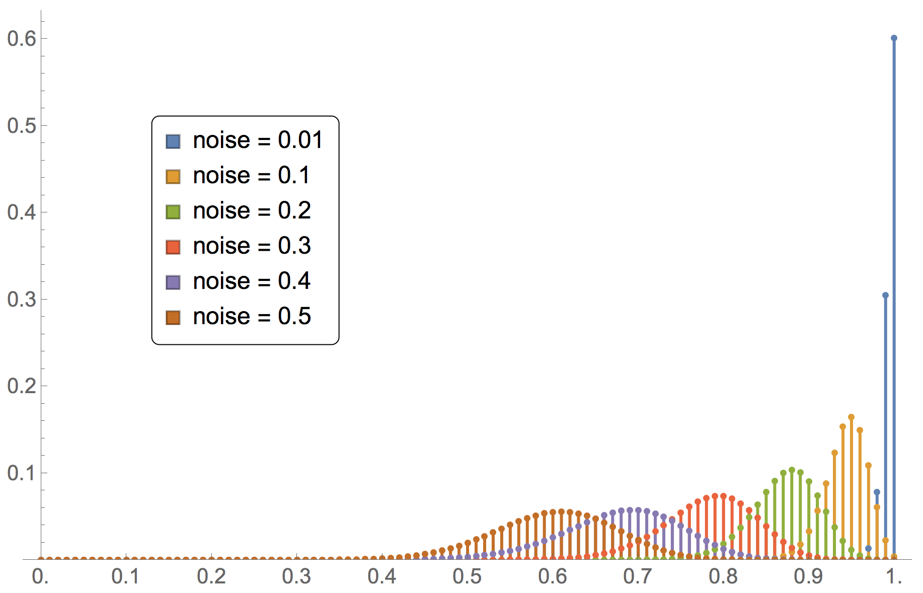
 for different values of noise in the coordination game [[1 0][0 2]] played by
  imitate-if-better agents
Figure 9 has been created by running the following Mathematica® script:
n = 100;

p[x_, noise_]:= (1-x)((1-noise)(x n/(n-1))((x n - 1)/(n-1)) + noise/2)
q[x_, noise_]:= x((1-noise)(((1-x)n)/(n-1))^2 ((1-x)n-1)/(n-1) + noise/2)

μs = Map[Normalize[
      FoldList[Times, 1, Table[p[(j-1)/n, #] / q[j/n, #], {j, n}]]
      , Total]&, {0.01, 0.1, 0.2, 0.3, 0.4, 0.5}];

ListPlot[μs, DataRange->{0, 1}, PlotRange->{0, All}, Filling -> Axis]
The limiting distribution of birth-death chains can be further characterized using results in Sandholm (2007).
3.2. Approximation results
In many models, a full Markov analysis cannot be conducted because the exact formulas are too complicated or because they may be too computationally expensive to evaluate. In such cases, we can still apply a variety of approximation results. This section introduces some of them.
3.2.1. Deterministic approximations of transient dynamics when the population is large. The mean dynamic
When the number of agents is sufficiently large, the mean dynamic of the process provides a good deterministic approximation to the dynamics of the stochastic evolutionary process over finite time spans. In this section we are going to analyze the behavior of our evolutionary process as the population size ![]() becomes large, so we make this dependency on
becomes large, so we make this dependency on ![]() explicit by using superscripts for
explicit by using superscripts for ![]() ,
, ![]() and
and ![]() .
.
Let us start by illustrating the essence of the mean dynamic approximation with our running example where ![]() imitate-if-better agents are playing the coordination game [[1 0][0 2]] without noise. Initially, half the agents are playing strategy 1 (i.e.
imitate-if-better agents are playing the coordination game [[1 0][0 2]] without noise. Initially, half the agents are playing strategy 1 (i.e. ![]() ). Figures 10, 11 and 12 show the expected proportion of 1-strategists
). Figures 10, 11 and 12 show the expected proportion of 1-strategists ![]() against the number of revisions
against the number of revisions ![]() (scaled by
(scaled by ![]() ), together with the 95% band for
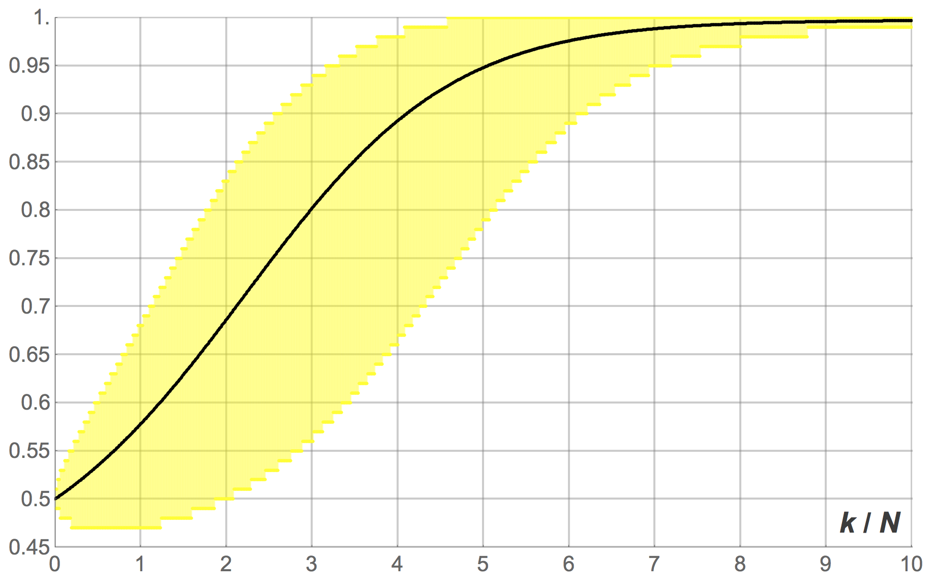
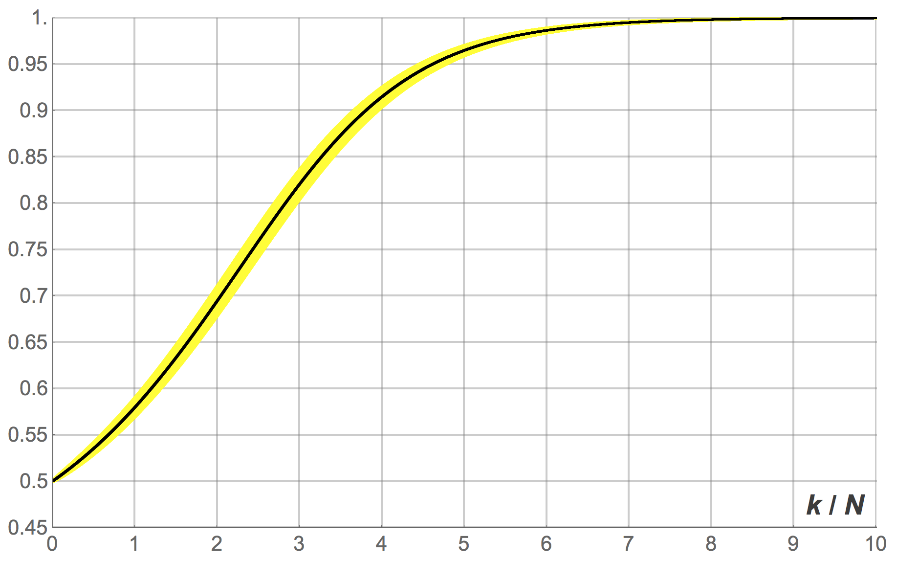
), together with the 95% band for ![]() , for different population sizes.[10] Figure 10 shows the transient dynamics for
, for different population sizes.[10] Figure 10 shows the transient dynamics for ![]() , figure 11 for
, figure 11 for ![]() and figure 12 for
and figure 12 for ![]() . These figures show exact results, computed as explained in section 3.1.2.
. These figures show exact results, computed as explained in section 3.1.2.
 imitate-if-better agents. Initially, half the population is using strategy 1
 imitate-if-better agents. Initially, half the population is using strategy 1
 imitate-if-better agents. Initially, half the population is using strategy 1
Looking at figures 10, 11 and 12 it is clear that, as the number of agents ![]() gets larger, the stochastc evolutionary process
gets larger, the stochastc evolutionary process ![]() gets closer and closer to its expected motion. The intuition is that, as the number of agents gets large, the fluctuations of the evolutionary process around its expected motion tend to average out. In the limit when
gets closer and closer to its expected motion. The intuition is that, as the number of agents gets large, the fluctuations of the evolutionary process around its expected motion tend to average out. In the limit when ![]() goes to infinity, the stochastic evolutionary process is very likely to behave in a nearly deterministic way, mirroring a solution trajectory of a certain ordinary differential equation called the mean dynamic.
goes to infinity, the stochastic evolutionary process is very likely to behave in a nearly deterministic way, mirroring a solution trajectory of a certain ordinary differential equation called the mean dynamic.
To derive the mean dynamic of our 2-strategy evolutionary process, we consider the behavior of the process ![]() over the next
over the next ![]() time units, departing from state
time units, departing from state ![]() . We define one unit of clock time as
. We define one unit of clock time as ![]() ticks, i.e. the time over which every agent is expected to receive exactly one revision opportunity. Thus, over the time interval
ticks, i.e. the time over which every agent is expected to receive exactly one revision opportunity. Thus, over the time interval ![]() , the number of agents who are expected to receive a revision opportunity is
, the number of agents who are expected to receive a revision opportunity is ![]() Of these
Of these ![]() agents who revise their strategies,
agents who revise their strategies, ![]() are expected to switch from strategy 0 to strategy 1 and
are expected to switch from strategy 0 to strategy 1 and ![]() are expected to switch from strategy 1 to strategy 0. Hence, the expected change in the number of agents that are using strategy 1 over the time interval
are expected to switch from strategy 1 to strategy 0. Hence, the expected change in the number of agents that are using strategy 1 over the time interval ![]() is
is ![]() . Therefore, the expected change in the proportion of agents using strategy 1, i.e. the expected change in state at
. Therefore, the expected change in the proportion of agents using strategy 1, i.e. the expected change in state at ![]() , is
, is
![]()
Note that the transition probabilities ![]() and
and ![]() may depend on
may depend on ![]() . This does not represent a problem as long as this dependency vanishes as
. This does not represent a problem as long as this dependency vanishes as ![]() gets large. In that case, to deal with that dependency, we take the limit of
gets large. In that case, to deal with that dependency, we take the limit of ![]() and
and ![]() as
as ![]() goes to infinity since, after all, the mean dynamic approximation is only valid for large
goes to infinity since, after all, the mean dynamic approximation is only valid for large ![]() . Thus, defining
. Thus, defining
![]()
and
![]()
we arrive at the mean dynamic equation:
![]()
As an illustration of the usefulness of the mean dynamic to approximate transient dynamics, consider the simulations of the coordination game example presented in section 2. We already computed the transition probabilities ![]() and
and ![]() in section 3.1.1:
in section 3.1.1:
![]()
![]()
Thus, the mean dynamic reads:
![]()
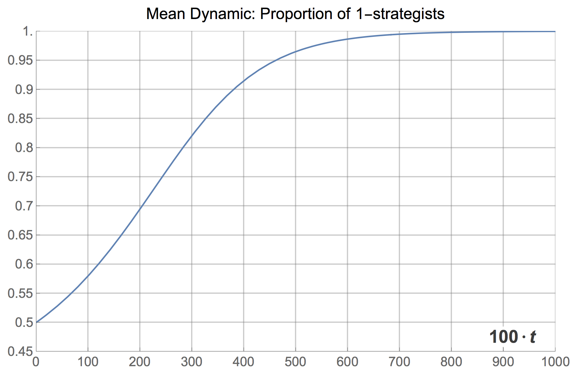
where ![]() stands for the fraction of 1-strategists. The solution of the mean dynamic with initial condition
stands for the fraction of 1-strategists. The solution of the mean dynamic with initial condition ![]() is shown in figure 13 below. It is clear that the mean dynamic provides a remarkably good approximation to the average transient dynamics plotted in figures 1 and 3.[11] And, as we have seen, the greater the number of agents, the closer the stochastic process will get to its expected motion.
is shown in figure 13 below. It is clear that the mean dynamic provides a remarkably good approximation to the average transient dynamics plotted in figures 1 and 3.[11] And, as we have seen, the greater the number of agents, the closer the stochastic process will get to its expected motion.
Naturally, the mean dynamic can be solved for many different initial conditions, providing an overall picture of the transient dynamics of the model when the population is large. Figure 14 below shows an illustration, created with the following Mathematica® code:
Plot[
 Evaluate[
  Table[
   NDSolveValue[{x'[t] == x[t] (x[t] - 1) (x[t]^2 - 3 x[t] + 1),
      x[0] == x0}, x, {t, 0, 10}][ticks/100]
  , {x0, 0, 1, 0.01}]
 ], {ticks, 0, 1000}]
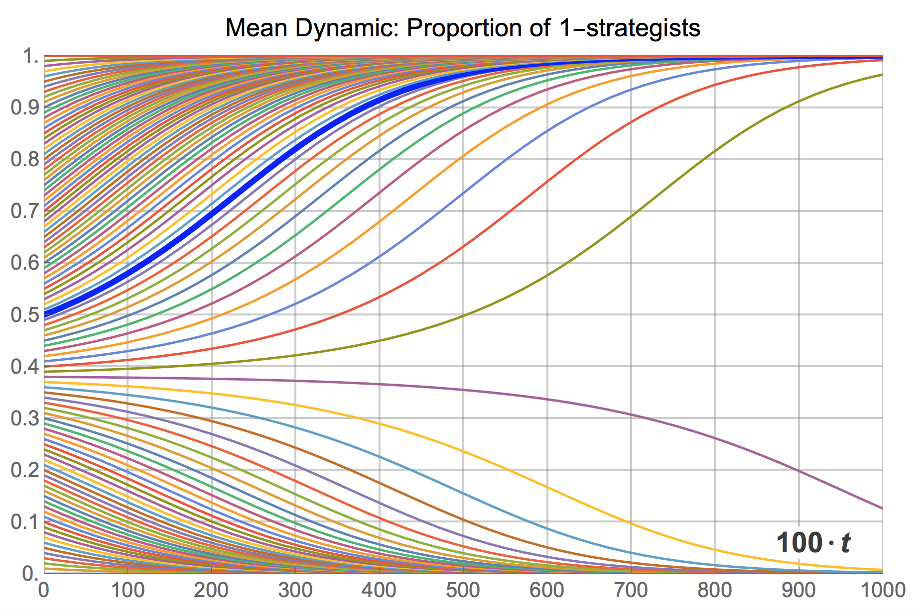
The cut-off point that separates the set of trajectories that go towards state ![]() from those that will end up in state
from those that will end up in state ![]() is easy to derive, by finding the rest points of the mean dynamic:
is easy to derive, by finding the rest points of the mean dynamic:
![]()
The three solutions in the interval ![]() are
are ![]() ,
, ![]() and
and ![]() .
.
In this section we have derived the mean dynamic for our 2-strategy evolutionary process where agents switch strategies sequentially. Note, however, that the mean dynamic approximation is valid for games with any number of strategies and even for models where several revisions take place simultaneously (as long as the number of revisions is fixed as ![]() goes to infinity or the probability of revision is
goes to infinity or the probability of revision is ![]() ).
).
It is also important to note that, even though here we have presented the mean dynamic approximation in informal terms, the link between the stochastic process and its relevant mean dynamic rests on solid theoretical grounds (see Benaïm & Weibull (2003), Sandholm (2010a, chapter 10) and Roth & Sandholm (2013)).
Finally, to compare agent-based simulations of the imitate-if-better rule and its mean dynamics in 2×2 symmetric games, you may want to play with the purpose-built demonstration titled Expected Dynamics of an Imitation Model in 2×2 Symmetric Games. And to solve the mean dynamic of the imitate-if-better rule in 3-strategy games, you may want to use this demonstration. In chapter V-3, we derive the mean dynamic for many other decision rules besides imitate-if-better, and we provide a NetLogo model that numerically solves the mean dynamic for different settings at runtime.
3.2.2. Diffusion approximations to characterize dynamics around equilibria
“Equilibria” in finite population dynamics are often defined as states where the expected motion of the (stochastic) process is zero. Formally, these equilibria correspond to the rest points of the mean dynamic of the original stochastic process. At some such equilibria, agents do not switch strategies anymore. Examples of such static equilibria would be the states where all agents are using the same strategy under the imitate-if-better rule. However, at some other equilibria, the expected flows of agents switching between different strategies cancel one another out (so the expected motion is indeed zero), but agents keep revising and changing strategies, potentially in a stochastic fashion. To characterize the dynamics around this second type of “equilibria”, which are most often interior, the diffusion approximation is particularly useful.
As an example, consider a Hawk-Dove game with payoffs [[2 1][3 0]] and the imitate-if-better decision rule without noise. The mean dynamic of this model is:
![]()
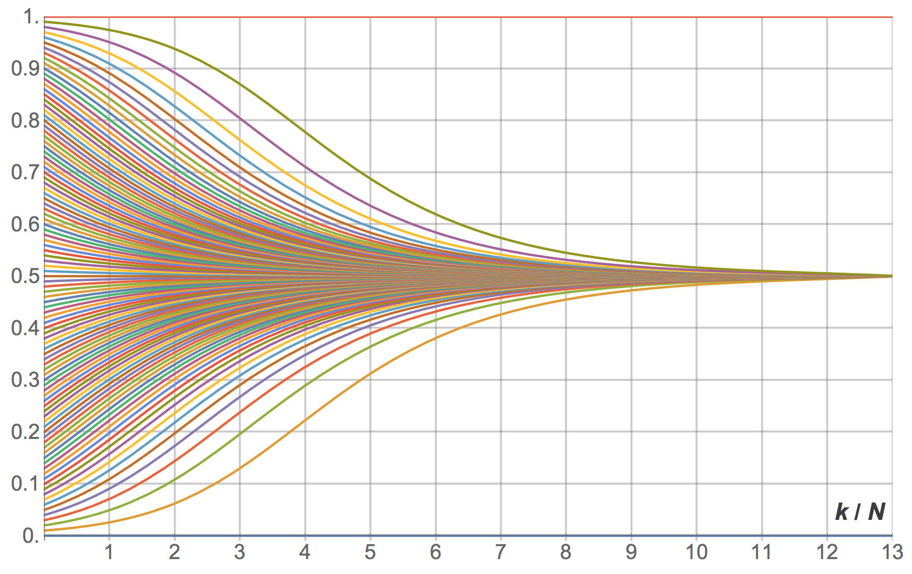
where ![]() stands for the fraction of 1-strategists, i.e. “Hawk” agents.[12] Solving the mean dynamic reveals that most large-population simulations starting with at least one “Hawk” and at least one “Dove” will tend to approach the state where half the population play “Hawk” and the other play “Dove”, and stay around there for long. Figure 15 below shows several trajectories for different initial conditions.
stands for the fraction of 1-strategists, i.e. “Hawk” agents.[12] Solving the mean dynamic reveals that most large-population simulations starting with at least one “Hawk” and at least one “Dove” will tend to approach the state where half the population play “Hawk” and the other play “Dove”, and stay around there for long. Figure 15 below shows several trajectories for different initial conditions.
 revisions
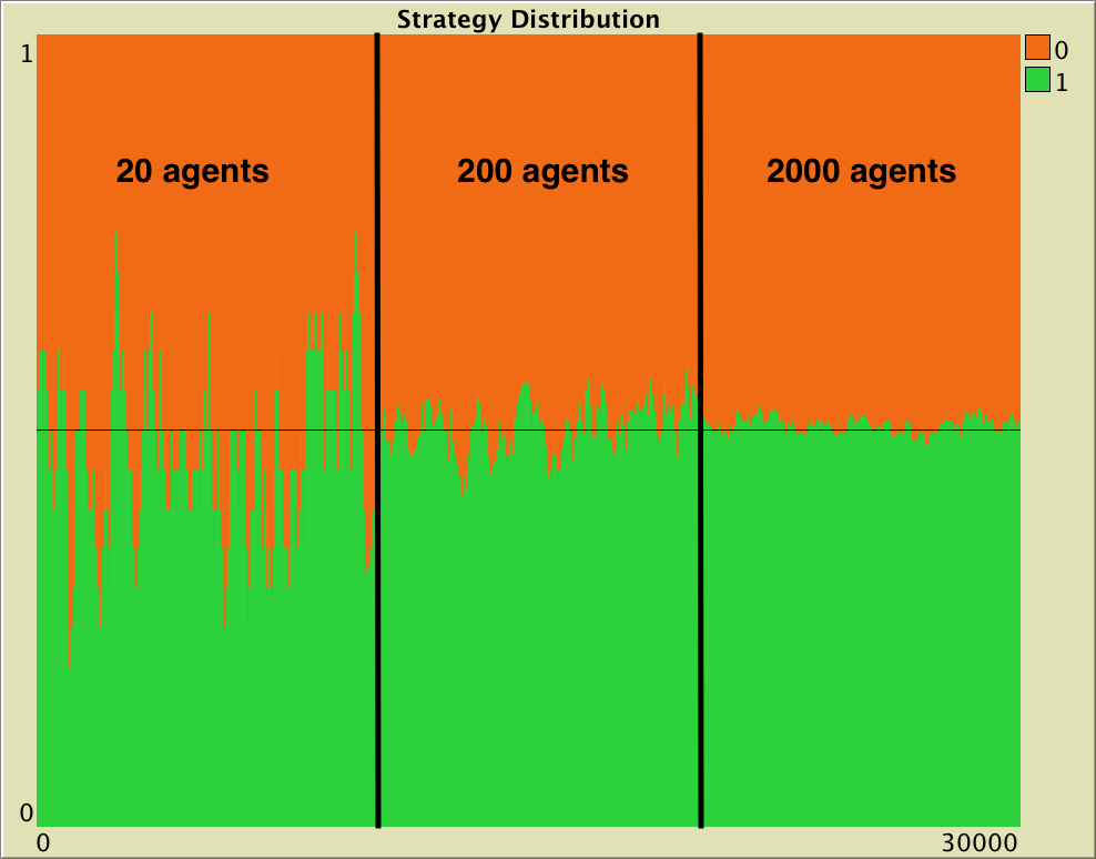
Naturally, simulations do not get stuck in the half-and-half state, since agents keep revising their strategy in a stochastic fashion (see figure 16). To understand this stochastic flow of agents between strategies near equilibria, it is necessary to go beyond the mean dynamic. Sandholm (2003) shows that –under rather general conditions– stochastic finite-population dynamics near rest points can be approximated by a diffusion process, as long as the population size ![]() is large enough. He also shows that the standard deviations of the limit distribution are of order
is large enough. He also shows that the standard deviations of the limit distribution are of order ![]() .
.
To illustrate this order ![]() , we set up one simulation run starting with 10 agents playing “Hawk” and 10 agents playing “Dove”. This state constitutes a so-called “Equilibrium”, since the expected change in the strategy distribution is zero. However, the stochasticity in the decision rule and in the matching process imply that the strategy distribution is in perpetual change. In the simulation shown in figure 16, we modify the number of players at runtime. At tick 10000, we increase the number of players by a factor of 10 up to 200 and, after 10000 more ticks, we set n-of-players to 2000 (i.e., a factor of 10, again). The standard deviation of the fraction of players using strategy “Hawk” (or “Dove”) during each of the three stages in our simulation run was: 0.1082, 0.0444 and 0.01167 respectively. As expected, these numbers are related by a factor of approximately
, we set up one simulation run starting with 10 agents playing “Hawk” and 10 agents playing “Dove”. This state constitutes a so-called “Equilibrium”, since the expected change in the strategy distribution is zero. However, the stochasticity in the decision rule and in the matching process imply that the strategy distribution is in perpetual change. In the simulation shown in figure 16, we modify the number of players at runtime. At tick 10000, we increase the number of players by a factor of 10 up to 200 and, after 10000 more ticks, we set n-of-players to 2000 (i.e., a factor of 10, again). The standard deviation of the fraction of players using strategy “Hawk” (or “Dove”) during each of the three stages in our simulation run was: 0.1082, 0.0444 and 0.01167 respectively. As expected, these numbers are related by a factor of approximately ![]() .
.
As a matter of fact, Izquierdo et al. (2019, example 3.1) use the diffusion approximation to show that in the large ![]() limit, fluctuations of this process around its unique interior rest point
limit, fluctuations of this process around its unique interior rest point ![]() are approximately Gaussian with standard deviation
are approximately Gaussian with standard deviation ![]() .
.
3.2.3. Stochastic stability analyses
In the last model we have implemented, if noise is strictly positive, the model’s infinite-horizon behavior is characterized by a unique stationary distribution regardless of initial conditions (see section 3.1 above). This distribution has full support (i.e. all states will be visited infinitely often) but, naturally, the system will spend much longer in certain areas of the state space than in others. If the noise is sufficiently small (but strictly positive), the infinite-horizon distribution of the Markov chain tends to concentrate most of its mass on just a few states. Stochastic stability analyses are devoted to identifying such states, which are often called stochastically stable states (Foster and Young, 1990), and are a subset of the absorbing states of the process without noise.[13]
To learn about this type of analysis, the following references are particularly useful: Vega-Redondo (2003, section 12.6), Fudenberg and Imhof (2008), Sandholm (2010a, chapters 11 and 12) and Wallace and Young (2015).
To illustrate the applicability of stochastic stability analyses, consider our imitate-if-better model where agents play the Hawk-Dove game analyzed in section 3.2.2 with some strictly positive noise. It can be proved that the only stochastically stable state in this model is the state where everyone chooses strategy Hawk.[14] This means that, given a certain population size, as noise tends to 0, the infinite-horizon dynamics of the model will concentrate on that single state.
An important concern in stochastic stability analyses is the time one has to wait until the prediction of the analysis becomes relevant. This time can be astronomically long, as the following example illustrates.
3.2.4 A final example
A fundamental feature of these models, but all too often ignored in applications, is that the asymptotic behavior of the short-run deterministic approximation need have no connection to the asymptotic behavior of the stochastic population process. Blume (1997, p. 443)
Consider the Hawk-Dove game analyzed in section 3.2.2, played by ![]() imitate-if-better agents with noise = 10-10, departing from an initial state where 28 agents are playing Hawk. Even though the population size is too modest for the mean dynamic and the diffusion approximations to be accurate, this example will clarify the different time scales at which each of the approximations is useful.
imitate-if-better agents with noise = 10-10, departing from an initial state where 28 agents are playing Hawk. Even though the population size is too modest for the mean dynamic and the diffusion approximations to be accurate, this example will clarify the different time scales at which each of the approximations is useful.
Let us review what we can say about this model using the three approximations discussed in the previous sections:
- Mean dynamic. Figure 15 shows the mean dynamic of this model without noise. The noise we are considering here is so small that the mean dynamic looks the same in the time interval shown in figure 15.[15] So, in our model with small noise, for large
 , the process will tend to move towards state
  , a journey that will take about
  revisions for our initial conditions
  . The greater the
  , the closer the stochastic process will be to the solution trajectory of its mean dynamic.
 - Diffusion approximation. Once in the vicinity of the unique interior rest point
 , the diffusion approximation tells us that –for large
  – the dynamics are well approximated by a Gaussian distribution with standard deviation
  .
. - Stochastic stability. Finally, we also know that, for a level of noise low enough (but strictly positive), the limiting distribution is going to place most of its mass on the unique stochastically stable state, which is
 . So, eventually, the dynamics will approach its limiting distribution, which –assuming the noise is low enough– places most of its mass on the monomorphic state
  .[16]
.[16]
Each of these approximations refers to a different time scale. In this regard, we find the classification made by Binmore and Samuelson (1994) and Binmore et al. (1995) very useful (see also Samuelson (1997) and Young (1998)). These authors distinguish between the short run, the medium run, the long run and the ultralong run:
By the short run, we refer to the initial conditions that prevail when one begins one’s observation or analysis. By the ultralong run, we mean a period of time long enough for the asymptotic distribution to be a good description of the behavior of the system. The long run refers to the time span needed for the system to reach the vicinity of the first equilibrium in whose neighborhood it will linger for some time. We speak of the medium run as the time intermediate between the short run [i.e. initial conditions] and the long run, during which the adjustment to equilibrium is occurring. Binmore et al. (1995, p. 10)
Let us see these different time scales in our Hawk-Dove example. The following video shows the exact transient dynamics of this model, computed as explained in section 3.1.2. Note that the video shows all the revisions up until ![]() , but then it moves faster and faster. The blue progress bar indicates the number of revisions already shown.
, but then it moves faster and faster. The blue progress bar indicates the number of revisions already shown.
Transient dynamics of a model where ![]() imitate-if-better agents are playing a Hawk-Dove game, with noise=
imitate-if-better agents are playing a Hawk-Dove game, with noise=![]() . Each iteration corresponds to one revision
. Each iteration corresponds to one revision
In the video we can distinguish the different time scales:
- The short run, which is determined by the initial conditions
 .
. - The medium run, which in this case spans roughly from
 to
to  . The dynamics of this adjustment process towards the equilibrium
  can be characterized by the mean dynamic, especially for large
  .
. - The long run, which in this case refers to the dynamics around the equilibrium
 , spanning roughly from
  to
to  . These dynamics are well described by the diffusion approximation, especially for large
  .
. - The ultra long run, which in this case is not really reached until
 . It is not until then that the limiting distribution becomes a good description of the dynamics of the model.
It is remarkable how long it takes for the infinite horizon prediction to hold force. Furthermore, the wait grows sharply as ![]() increases and also as the level of noise decreases.[17] These long waiting times are typical of stochastic stability analyses, so care must be taken when applying the conclusions of these analyses to real world settings.
increases and also as the level of noise decreases.[17] These long waiting times are typical of stochastic stability analyses, so care must be taken when applying the conclusions of these analyses to real world settings.
In summary, as ![]() grows, both the mean dynamic and the difussion approximations become better. For any fixed
grows, both the mean dynamic and the difussion approximations become better. For any fixed ![]() , eventually, the behavior of the process will be well described by its limiting distribution. If the noise is low enough (but strictly positive), the limiting distribution will place most of its mass on the unique stochastically stable state
, eventually, the behavior of the process will be well described by its limiting distribution. If the noise is low enough (but strictly positive), the limiting distribution will place most of its mass on the unique stochastically stable state ![]() . But note that, as
. But note that, as ![]() grows, it will take exponentially longer for the infinite-horizon prediction to kick in (see Sandholm and Staudigl (2018)).
grows, it will take exponentially longer for the infinite-horizon prediction to kick in (see Sandholm and Staudigl (2018)).
Note also that for the limiting distribution to place most of its mass on the stochastically stable state, the level of noise has to be sufficiently low, and if the population size ![]() increases, the maximum level of noise at which the limiting distribution concentrates most of its mass on the stochastically stable state decreases. As an example, consider the same setting as the one shown in the video, but with
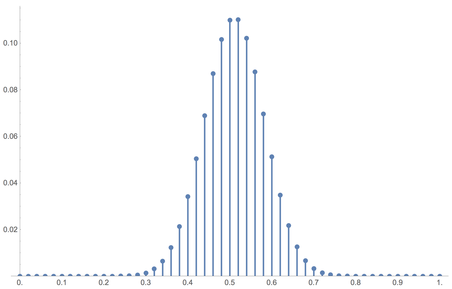
increases, the maximum level of noise at which the limiting distribution concentrates most of its mass on the stochastically stable state decreases. As an example, consider the same setting as the one shown in the video, but with ![]() . In this case, the limiting distribution is completely different (see figure 17). A noise level of 10-10 is not enough for the limiting distribution to place most of its mass on the stochastically stable state when
. In this case, the limiting distribution is completely different (see figure 17). A noise level of 10-10 is not enough for the limiting distribution to place most of its mass on the stochastically stable state when ![]() .
.
 imitate-if-better agents are playing a Hawk-Dove game, with noise = 10-10
Figure 17 has been created by running the following Mathematica® script:
n = 50;
noise = 10^-10;

p[x_, noise_] := (1-x)((1-noise)((x n)/(n-1))((1-x)n/(n-1)) + noise/2)
q[x_, noise_] := x((1-noise)(((1-x)n)/(n-1))(x n - 1)/(n-1) + noise/2)

μ = Normalize[
      FoldList[Times, 1,
        Table[p[(j-1)/n, noise] / q[j/n, noise],{j, n}]]
     , Total];

ListPlot[μ, DataRange->{0, 1}, PlotRange->{0, All}, Filling -> Axis]
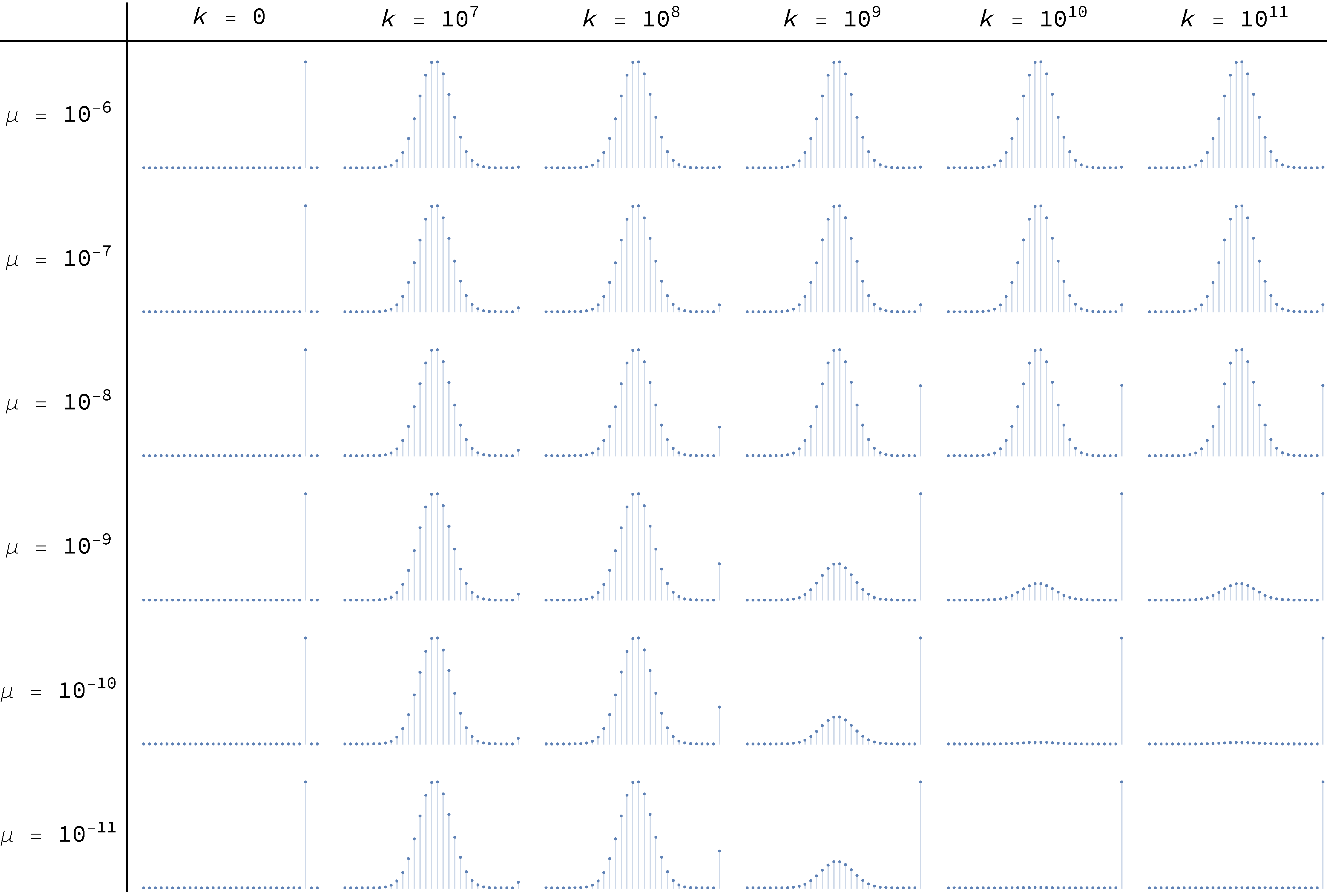
To conclude, Figure 18 and Figure 19 below show the transient distributions of this model with ![]() and
and ![]() respectively, for different levels of noise μ, and at different ticks
respectively, for different levels of noise μ, and at different ticks ![]() . The distributions at the far right, for
. The distributions at the far right, for ![]() , are effectively equal to the asymptotic ones.
, are effectively equal to the asymptotic ones.
 imitate-if-better agents are playing a Hawk-Dove game, with different levels of noise μ, and at different ticks
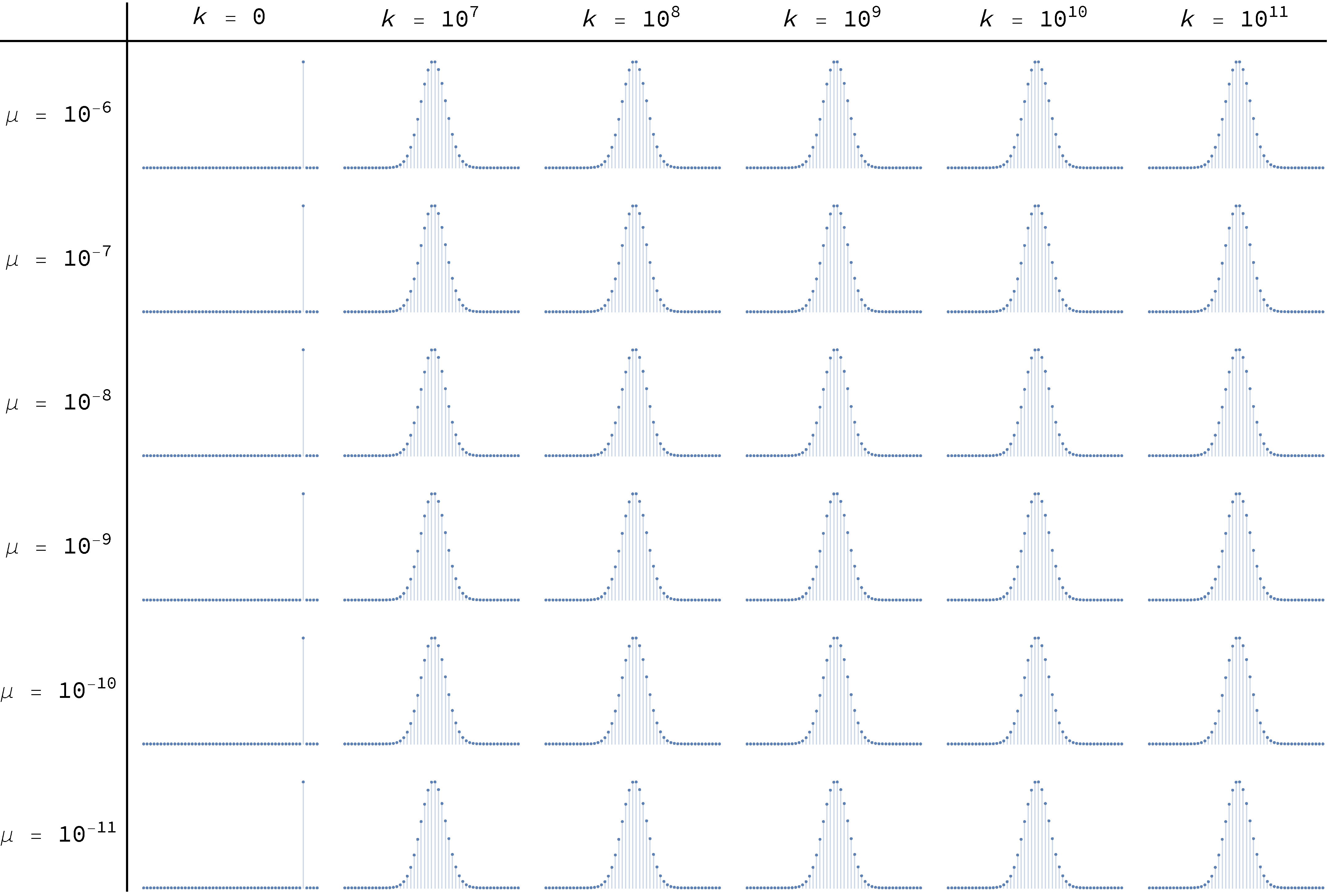
 imitate-if-better agents are playing a Hawk-Dove game, with different levels of noise μ, and at different ticks
Figure 18 and Figure 19 have been created by running the following Mathematica® script:
n = 30;

noiseLevels = Table[10^(-i), {i, 6, 11}];
ticks = Join[{0}, Table[10^i, {i, 7, 11}]];

initialDistribution = UnitVector[n + 1, Round[0.93*n] + 1];

p[x_, noise_] := (1-x)((1-noise)((x n)/(n-1))((1-x)n/(n-1)) + noise/2)
q[x_, noise_] := x((1-noise)(((1-x)n)/(n-1))(x n - 1)/(n-1) + noise/2)

P[noise_] := SparseArray[{
    {i_, i_} -> (1 - p[(i - 1)/n, noise] - q[(i - 1)/n, noise]),
    {i_, j_} /; i == j - 1 -> p[(i - 1)/n, noise],
    {i_, j_} /; i == j + 1 -> q[(i - 1)/n, noise]},
    {n + 1, n + 1}];

FormatNice[i_]:=
  If[i == 0., 0, ScientificForm[N@i, NumberFormat -> (10^#3 &)]];

TableForm[
 Table[
  ListPlot[
   initialDistribution . MatrixPower[N@P[noise], finalTimestep],
   Filling -> Axis, PlotRange -> All, ImageSize -> Tiny, Axes -> False],
  {noise, noiseLevels}, {finalTimestep, ticks}
  ],
 TableHeadings -> {
   Map[Row[{"μ = ", FormatNice[#]}] &, noiseLevels],
   Map[Row[{"k = ", FormatNice[#]}] &, ticks]},
 TableAlignments -> Center, TableSpacing -> {3, 1}]
4. Exercises
Exercise 1. Consider the evolutionary process analyzed in section 3.1.2. Figure 5 shows that, if we start with half the population using each strategy, the probability that the whole population will be using strategy 1 after 500 revisions is about 6.66%. Here we ask you to use the NetLogo model implemented in the previous chapter to estimate that probability. To do that, you will have to set up and run an experiment using BehaviorSpace.
Exercise 2. Derive the mean dynamic of a Prisoner’s Dilemma game for the imitate if better rule.
Exercise 3. Derive the mean dynamic of the coordination game discussed in chapter I-2 (with payoffs [[1 0][0 2]]) for the imitative pairwise-difference rule.
Exercise 4. Derive the mean dynamic of the coordination game discussed in chapter I-2 (with payoffs [[1 0][0 2]]) for the best experienced payoff rule.
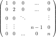
Exercise 5. For the best experienced payoff rule, derive the mean dynamic of the 2-player n-strategy (single-optimum) coordination game with the following payoff matrix:
Exercise 6. Once you have done exercise 5 above, prove that, in the derived mean dynamics, the state where every player chooses the efficient strategy (which provides a payoff of n) attracts all trajectories except possibly those starting at the other monomorphic states in which all players use the same strategy.
- The standard error of the average equals the standard deviation of the sample divided by the square root of the sample size. In our example, the maximum standard error was well below 0.01. ↵
- This result can be easily derived using a "stars and bars" analogy. ↵
- As an example, in a 4-strategy game with 1000 players, the number of possible states (i.e. strategy distributions) is
 . ↵
. ↵ - We give you a hint to program the asynchronous model in exercise 4 of chapter II-4. ↵
- These probabilities are sometimes called "fixation probabilities". ↵
- In terms of the transition probabilities
 and
and  , adding noise implies that
  for
for  (i.e. you can always move one step to the right unless
  already equals 1),
  for
for  (i.e. you can always move one step to the left unless
  already equals 0) and
  for all
 ![Rendered by QuickLaTeX.com x \in [0,1]](https://wisc.pb.unizin.org/app/uploads/quicklatex/quicklatex.com-7d1a4c305481e63e6e4d63033a4f70d0_l3.png) (i.e. you can always stay where you are). ↵
(i.e. you can always stay where you are). ↵ - Formally, the occupancy of state
 is defined as:
where
 denotes the number of times that the Markov chain visits state
  over the time span
  . ↵
. ↵ - The second-largest eigenvalue modulus of the transition matrix
 determines the rate of convergence to the limiting distribution. ↵
 - For the derivation of this formula, see e.g. Sandholm (2010a, example 11.A.10, p. 443). ↵
- For each value of
 , the band is defined by the smallest interval
  that leaves less than 2.5% probability at both sides, i.e.
  and
and  , with
  . ↵
. ↵ - Note that one unit of clock time in the mean dynamic is defined in such a way that each player expects to receive one revision opportunity per unit of clock time. In the model simulated in section 2, prob-revision = 0.01, so one unit of clock time corresponds to 100 ticks (i.e. 1 / prob-revision). ↵
- For details, see Izquierdo and Izquierdo (2013) and Loginov (2021). ↵
- There are a number of different definitions of stochastic stability, depending on which limits are taken and in what order. For a discussion of different definitions, see Sandholm (2010a, chapter 12). ↵
- To be precise, here we are considering stochastic stability in the small noise limit, where we fix the population size and take the limit of noise to zero (Sandholm, 2010a, section 12.1.1). The proof can be conducted using the concepts and theorems put forward by Ellison (2000). Note that the radius of the state where everyone plays Hawk is 2 (i.e. 2 mutations are needed to leave its basin of attraction), while its coradius is just 1 (one mutation is enough to go from the state where everyone plays Dove to the state where everyone plays Hawk). ↵
- The only difference is that, in the model with noise, the two trajectories starting at the monomorphic states eventually converge to the state
 , but this convergence cannot be appreciated in the time interval shown in figure 15. ↵
 - Using the analytic formula for the limiting distribution of irreducible and aperiodic birth-death chains provided in section 3.1.3, we have checked that
 for
for  and noise = 10-10. ↵
 - Using tools from large deviations theory, Sandholm and Staudigl (2018) show that –for large population sizes
 – the time required to reach the boundary is of an exponential order in
  . ↵
. ↵

