Part IV. Games on networks
IV-3. Implementing network metrics
1. Goal
Our goal in this chapter is to include some network metrics in our model. These metrics will give us information about the structure of the generated network. In particular, we will compute:
- The network density, which is the number of links present in the network divided by the total number of links that could exist.
- The size of the largest component. A component is a maximal set of connected nodes, i.e. a maximal group of nodes such that there is a path from each node to every other node.
- The average local clustering coefficient. The local clustering coefficient of a node is the number of existing links between its neighbors divided by the total number of links that could possibly exist between them.[1] In a social network of friendships, this metric would measure the extent to which your friends are friends among themselves.
- The degree distribution, which shows the number of nodes that have degree k (with k = 0, 1, 2, 3…). As an example, figure 1 below shows the degree distribution of various networks with 100 nodes.[2]
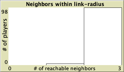
Path network (2 at 1; 98 at 2) 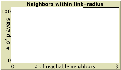
Ring network (100 at 2) 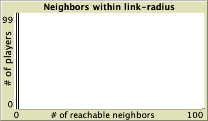
Star network (99 at 1; 1 at 99) 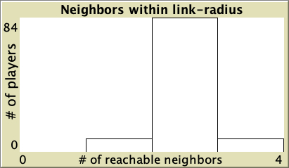
Watts-Strogatz small-world network with average degree 2 and probability of rewiring = 0.1 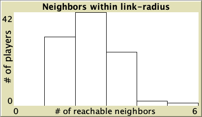
Watts-Strogatz small-world network with average degree 2 and probability of rewiring = 0.5 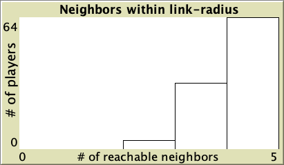
10×10 square grid network (4 at 2; 32 at 3; 64 at 4) 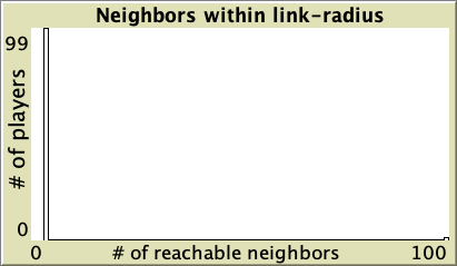
Wheel network (99 at 3; 1 at 99) Figure 1. Degree distribution of different types of networks with 100 nodes
Note that the degree of a node is the number of nodes that are at (geodesic) distance 1; in our model we will also compute the number of nodes that are within distances greater than 1.
2. Motivation. Reassessing the significance of network structure
Let us revisit the 2-player 2-strategy single-optimum coordination game of the previous chapter:
| Player 2 | |||
| Player 2 chooses A | Player 2 chooses B | ||
| Player 1 | Player 1 chooses A | 1 , 1 | 0 , 0 |
| Player 1 chooses B | 0 , 0 | 2 , 2 | |
In the previous chapter we saw that, in this game, under certain conditions,[3] a population of 100 agents embedded on a network with average degree about 2, will most likely approach the state where all agents choose strategy B and spend most of the time close to it, regardless of the network structure. The star network was an exception, but the result seems to hold for most network structures. Network structure did not seem to play a significant role in networks with very high density either; in those networks, given our conditions, agents tend to approach the inefficient state and spend most of the time around there.
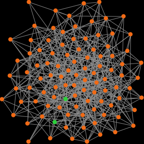
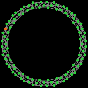
However, for moderately low densities (e.g. average degree about 10), network structure clearly plays a role, as you can see in the figures below. Figures 2 and 3 show two networks with average degree about 10, but completely different structure. Figure 2 shows a random network generated with the Erdős–Rényi model, and figure 3 shows a ring lattice. In the random network, most simulation runs approach the inefficient state and stay around it, while in the ring lattice, most simulations approach and stay around the efficient state.
 |
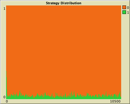 |
Figure 2. On the left, an Erdős–Rényi random network with average degree about 10 (prob-link = 0.1). On the right, a representative run of our model in that network
 |
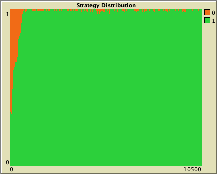 |
Figure 3. On the left, a ring lattice where all players have degree 10, generated using the Watts–Strogatz model with prob-rewiring = 0. On the right, a representative run of our model in that network
For those cases where the average degree is certainly not enough to predict whether the population will approach the efficient state or not, we would like to explore whether there is any other property of the network that may help us predict the most likely outcome of the simulation. In particular, we hypothesize that the average local clustering coefficient may be useful, since this is a metric that is very different in the two networks shown in figures 2 and 3. For sufficiently large networks, the local clustering coefficient in Erdős–Rényi random networks is about prob-link for every node (so it is about 0.1 in the random network above),[4] while it is exactly ![]() for all nodes in ring lattices of degree
for all nodes in ring lattices of degree ![]() (so it is exactly 2/3 ≈ 0.67 in the ring lattice above). So, does clustering help to approach the efficient state in our model?
(so it is exactly 2/3 ≈ 0.67 in the ring lattice above). So, does clustering help to approach the efficient state in our model?
Let us extend our model to explore this question!
3. Description of the model
We will not make any modification on the formal model our program implements. Thus, we refer you to the previous chapter to read the description of the model. The only paragraph we should add (about the program itself) is the following:
The program computes the following metrics for the generated network:
- The network density
- The size of the largest component.
- The average local clustering coefficient.
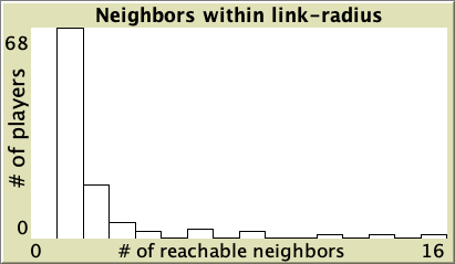
- The histogram for the number of players within distance link-radius (which is a new parameter in the model). If link-radius = 1, this histogram shows the degree distribution. If link-radius = 2, the histogram gives information about how many players can be reached through 2 or fewer links. In general, this histogram shows the number of players that have k other players within distance link-radius (with k = 0, 1, 2, 3…).
- The average number of (other) players within distance link-radius.
 4. Interface design
We depart from the model we developed in the previous chapter (so if you want to preserve it, now is a good time to duplicate it).
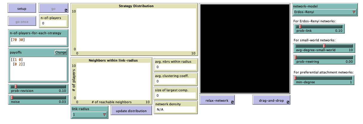
The new interface (see figure 4 above) includes a new plot, a new chooser, a new button and four new monitors, all of them placed below the “Strategy Distribution” plot. To be precise, we have to add:
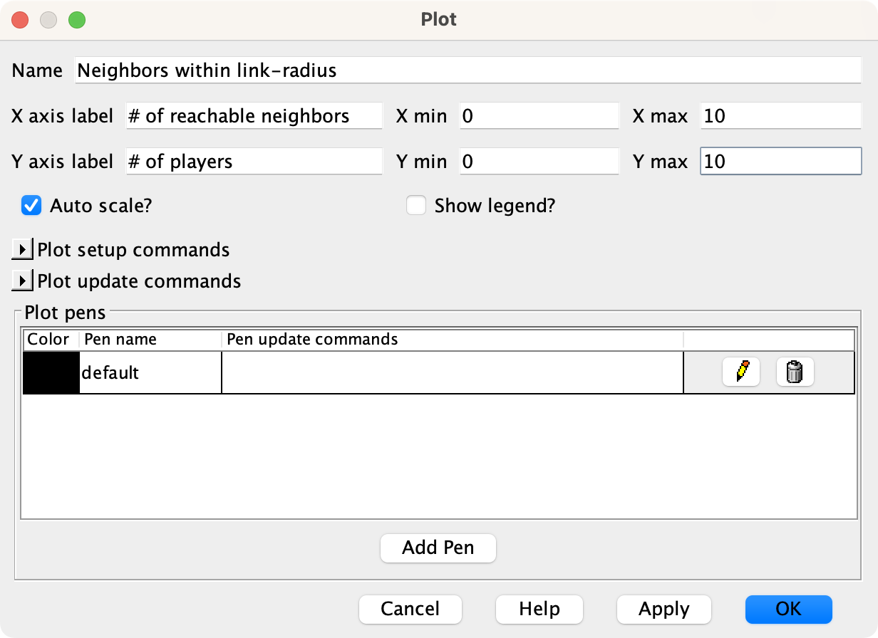
- One plot for the histogram. The horizontal axis should show the number of reachable neighbors (i.e., neighbors within distance link-radius) and the vertical axis should show how many players have the corresponding number of reachable neighbors.
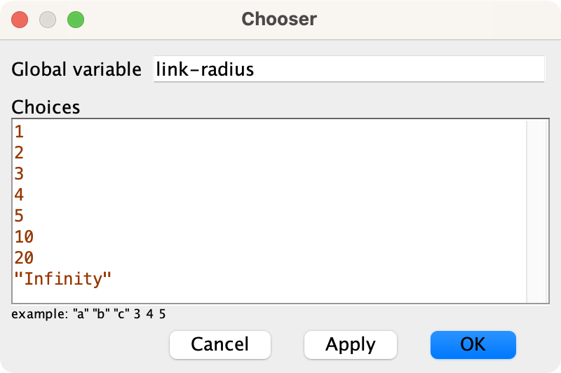
- One chooser for new parameter link-radius, with possible values 1, 2, 3, 4, 5, 10, 20 and “Infinity”.
- One button, to update the histogram.
In the Code tab, let us write the procedure to plot-accessibility, without including any code inside for now. This procedure will be in charge of updating the histogram.
to plot-accessibility
  ;; empty for now
end
Now we can create the button to run plot-accessibility. The user will have to click on this button after changing the value of parameter link-radius, so the new distribution is computed. Since this button only deals with informational aspects of the model, you may want to use the primitive with-local-randomness, which guarantees that this piece of code does not interfere with the generation of pseudorandom numbers for the rest of the model.
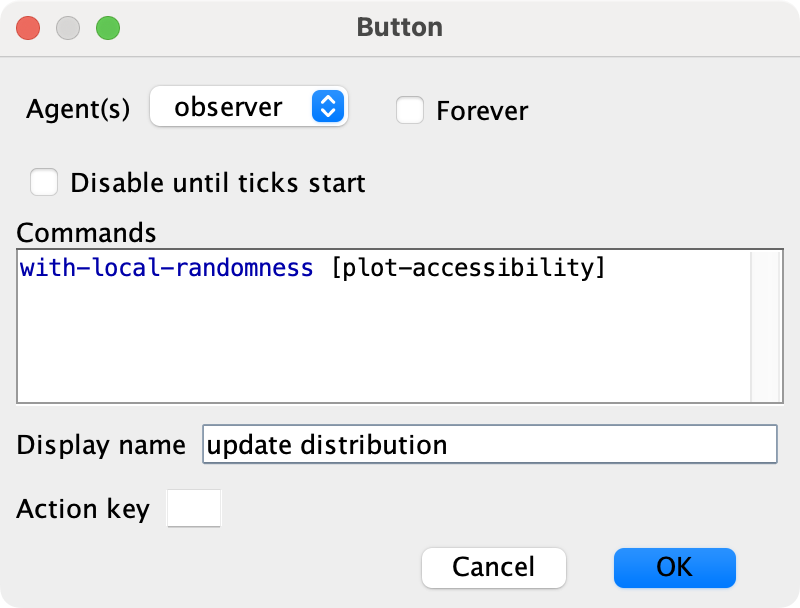
Settings for the button to update plot “Neighbors within link-radius” - Four monitors
1. Let us create a monitor to show the average number of neighbors within distance link-radius. We will store this value in a new global variable named avg-nbrs-within-radius. Thus, before creating the monitor, please add this new global variable in the Code tab.
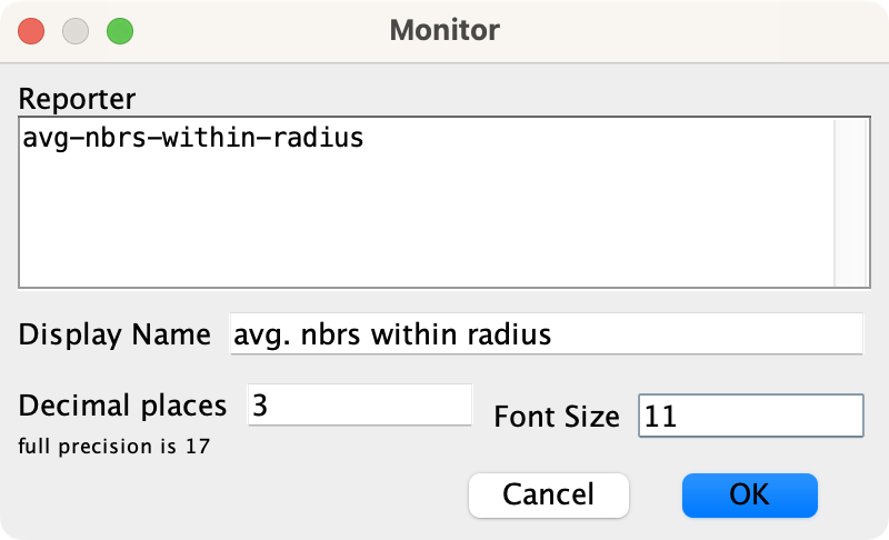
Settings for the monitor of global variable avg-nbrs-within-radius 2. Let us create a monitor to show the average local clustering coefficient. We will store this value in a new global variable named avg-clustering-coefficient. Thus, before creating the monitor, please add this new global variable in the Code tab.
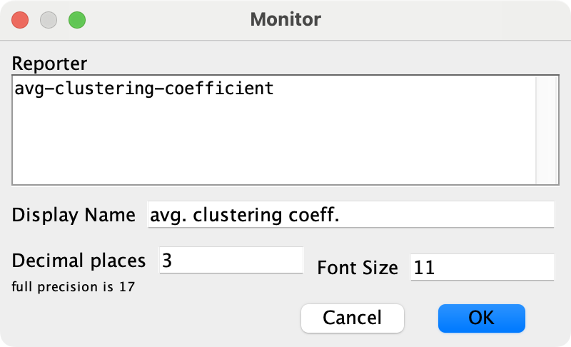
Settings for the monitor of global variable avg-clustering-coefficient 3. Let us create a monitor to show the size of the largest component. We will store this value in a new global variable named size-of-largest-component. Thus, before creating the monitor, please add this new global variable in the Code tab.

Settings for the monitor of global variable size-of-largest-component 4. And finally, let us create a monitor to show the network density. The maximum number of undirected links in a
 -node simple network is
  , so the density of a simple undirected network with
  links is
  .[5] Since the formula to compute the density is very simple, we can write it up directly in the monitor window.
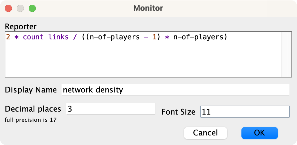
Settings for the monitor of the network density
 5. Code
5.1. Skeleton of the code
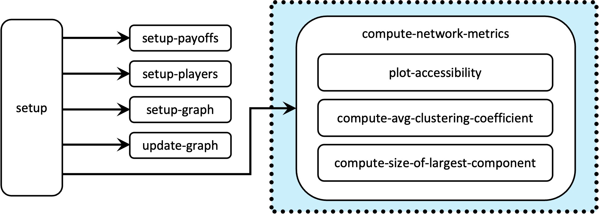
To keep our code beautiful and tidy, we will gather all the computations of the network metrics in a new procedure named to compute-network-metrics. It makes sense to run this new procedure soon after the network has been created, in procedure to setup (see fig. 5), since the network does not change over the course of the simulation. Procedure to compute-network-metrics will call three new procedures:
- to plot-accessibility, which will compute and show the histogram for the number of players within distance link-radius, and will also set the value of avg-nbrs-within-radius.
- to compute-avg-clustering-coefficient, which will compute the value of avg-clustering-coefficient.
- to compute-size-of-largest-component, which will compute the value of size-of-largest-component.
5.2. Global variables and individually-owned variables
Global variables
If you have already added global variables avg-nbrs-within-radius, avg-clustering-coefficient, and size-of-largest-component, then there is no need to add or remove any other global variables in our code. The current global variables are:
globals [
  payoff-matrix
  n-of-strategies
  n-of-players

  avg-nbrs-within-radius      ;; <== new line
  avg-clustering-coefficient  ;; <== new line
  size-of-largest-component   ;; <== new line
]
Individually-owned variables
There is no need to add or remove any individually-owned variables in our code.
5.3. Procedure to compute-network-metrics
Procedure to compute-network-metrics is just a container that gathers all the procedures in charge of computing the different network metrics (see fig. 5). We use this container to keep our code nice and modular. Its implementation is particularly simple:
to compute-network-metrics
  plot-accessibility
  compute-avg-clustering-coefficient
  compute-size-of-largest-component
end
As shown in fig. 5, we should call this new procedure at the end of setup:
to setup
  clear-all
  setup-payoffs
  setup-players
  setup-graph
  reset-ticks
  update-graph
  compute-network-metrics  ;; <== new line
end
5.4. Procedures to compute network metrics
In this section we implement the three procedures that compute the different network metrics.
to plot-accessibility
This procedure should compute and plot the accessibility histogram (i.e. the “Neighbors within link-radius” histogram). To do this, the reporter nw:turtles-in-radius is very useful, since it returns the set of neighbors that are within a certain (geodesic) distance of the calling player in the network. Thus, we just have to count the number of neighbors in this set for every player, after having set the required radius to link-radius:
to plot-accessibility

  let n-of-nbrs-of-each-player
    [(count nw:turtles-in-radius link-radius) - 1] of players
      ;; - 1 because nw:turtles-in-radius includes the calling player

end
Note, however, that parameter link-radius may take the value “Infinity”, to see the number of players that players can reach through any number of links. To compute this, note that the greatest possible distance between any two players connected in the network is the number of players in the network minus 1. Thus, if link-radius equals “Infinity”, we may call reporter nw:turtles-in-radius with the value of (n-of-players – 1). To implement this elegantly, we define a local variable named steps, as follows.
to plot-accessibility
  let steps link-radius
  if link-radius = "Infinity" [set steps (n-of-players - 1)]

  let n-of-nbrs-of-each-player
    [(count nw:turtles-in-radius steps) - 1] of players
      ;; - 1 because nw:turtles-in-radius includes the calling player
end
Now that we have the list of the number of reachable neighbors for each player, we can plot the histogram using the histogram command. Note, however, that there is an issue we have to be careful about when using histogram. In the produced histogram, the height of the bin that goes from x to (x+1) will be the frequency of all the values in the range [x, x+1), which in this case is just the integer value x. Thus, to include a bin for the maximum value in the list, we should set the upper limit of the horizontal range of the plot to the maximum value of the list plus 1. If we do not add this 1, we will not see the bin corresponding to the maximum number in the list.
Finally, in this procedure we should also compute the mean of the distribution and store it in global variable avg-nbrs-within-radius.
to plot-accessibility
  let steps link-radius
  if link-radius = "Infinity" [set steps (n-of-players - 1)]
  let n-of-nbrs-of-each-player
    [(count nw:turtles-in-radius steps) - 1] of players

  let max-n-of-nbrs-of-each-player max n-of-nbrs-of-each-player
  set-current-plot "Neighbors within link-radius"
  set-plot-x-range 0 (max-n-of-nbrs-of-each-player + 1)
                         ;; + 1 to make room for the width of the last bar
  histogram n-of-nbrs-of-each-player
  set avg-nbrs-within-radius mean n-of-nbrs-of-each-player
end
to compute-avg-clustering-coefficient
Have a look at the documentation of reporter nw:clustering-coefficient and try to implement this procedure.
Implementation of procedure to compute-avg-clustering-coefficient
to compute-avg-clustering-coefficient
  set avg-clustering-coefficient
      mean [ nw:clustering-coefficient ] of players
end
to compute-size-of-largest-component
Have a look at the documentation of reporter nw:weak-component-clusters and try to implement this procedure.
Implementation of procedure to compute-size-of-largest-component
to compute-size-of-largest-component
  set size-of-largest-component max map count nw:weak-component-clusters
end
5.5. Other procedures
Note that there is no need to modify the code of any other procedure.
5.6. Complete code in the Code tab
We have finished our model!
extensions [nw]

globals [
  payoff-matrix
  n-of-strategies
  n-of-players

  avg-nbrs-within-radius
  avg-clustering-coefficient
  size-of-largest-component
]

breed [players player]

players-own [
  strategy
  strategy-after-revision
  payoff
]

;;;;;;;;;;;;;
;;; SETUP ;;;
;;;;;;;;;;;;;

to setup
  clear-all
  setup-payoffs
  setup-players
  setup-graph
  reset-ticks
  update-graph
  compute-network-metrics
end

to setup-payoffs
  set payoff-matrix read-from-string payoffs
  set n-of-strategies length payoff-matrix
end

to setup-players
  let initial-distribution
      read-from-string n-of-players-for-each-strategy

  if length initial-distribution != length payoff-matrix [
    user-message (word "The number of items in\n"
      "n-of-players-for-each-strategy (i.e. "
      length initial-distribution "):\n"
      n-of-players-for-each-strategy
      "\nshould be equal to the number of rows\n"
      "in the payoff matrix (i.e. "
      length payoff-matrix "):\n"
      payoffs
    )
  ]

  set n-of-players sum initial-distribution
  ifelse n-of-players < 4
    [ user-message "There should be at least 4 players" ]
    [
      build-network

      ask players [set strategy -1]
      let i 0
      foreach initial-distribution [ j ->
        ask up-to-n-of j players with [strategy = -1] [
          set payoff 0
          set strategy i
          set strategy-after-revision strategy
        ]
        set i (i + 1)
      ]

      set n-of-players count players
      update-players-color
    ]
end

;;;;;;;;;;;;;;;;;;;;;;;;;;;;
;;; NETWORK CONSTRUCTION ;;;
;;;;;;;;;;;;;;;;;;;;;;;;;;;;

to build-network
  set-default-shape players "circle"
  run (word "build-" network-model "-network")
  ask players [fd 15]
end

to build-Erdos-Renyi-network
  nw:generate-random players links n-of-players
     prob-link
end

to build-Watts-Strogatz-small-world-network
 nw:generate-watts-strogatz players links n-of-players
    (avg-degree-small-world / 2) prob-rewiring
end

to build-preferential-attachment-network
  nw:generate-preferential-attachment players links n-of-players
     min-degree
end

to build-ring-network
  nw:generate-ring players links n-of-players
end

to build-star-network
  nw:generate-star players links n-of-players
end

to build-grid-4-nbrs-network
  let players-per-line (floor sqrt n-of-players)
  nw:generate-lattice-2d players links
     players-per-line players-per-line false
end

to build-wheel-network
  nw:generate-wheel players links n-of-players
end

to build-path-network
  build-ring-network
  ask one-of links [die]
end

;;;;;;;;;;
;;; GO ;;;
;;;;;;;;;;

to go
  ask players [update-payoff]
  ask players [
    if (random-float 1 < prob-revision) [
      update-strategy-after-revision
    ]
  ]
  ask players [update-strategy]

  tick
  update-graph
  update-players-color
end

;;;;;;;;;;;;;;;;;;;;;;;;;
;;; UPDATE PROCEDURES ;;;
;;;;;;;;;;;;;;;;;;;;;;;;;

to update-payoff
  if any? link-neighbors [
    let mate one-of link-neighbors
    set payoff
        item ([strategy] of mate) (item strategy payoff-matrix)
  ]
end

to update-strategy-after-revision
  ifelse random-float 1 < noise
    [ set strategy-after-revision (random n-of-strategies) ]
    [
      if any? link-neighbors [
        let observed-player one-of link-neighbors
        if ([payoff] of observed-player) > payoff [
          set strategy-after-revision
              ([strategy] of observed-player)
        ]
      ]
    ]
end

to update-strategy
  set strategy strategy-after-revision
end

;;;;;;;;;;;;;
;;; PLOTS ;;;
;;;;;;;;;;;;;

to setup-graph
  set-current-plot "Strategy Distribution"
  foreach (range n-of-strategies) [ i ->
    create-temporary-plot-pen (word i)
    set-plot-pen-mode 1
    set-plot-pen-color 25 + 40 * i
  ]
end

to update-graph
  let strategy-numbers (range n-of-strategies)
  let strategy-frequencies map [ n ->
        count players with [strategy = n] / n-of-players
      ] strategy-numbers

  set-current-plot "Strategy Distribution"
  let bar 1
  foreach strategy-numbers [ n ->
    set-current-plot-pen (word n)
    plotxy ticks bar
    set bar (bar - (item n strategy-frequencies))
  ]
  set-plot-y-range 0 1
end

to update-players-color
  ask players [set color 25 + 40 * strategy]
end

;;;;;;;;;;;;;;;;;;;;;;;
;;; NETWORK METRICS ;;;
;;;;;;;;;;;;;;;;;;;;;;;

to compute-network-metrics
  plot-accessibility
  compute-avg-clustering-coefficient
  compute-size-of-largest-component
end

to plot-accessibility
  let steps link-radius
  if link-radius = "Infinity" [set steps (n-of-players - 1)]
  let n-of-nbrs-of-each-player
    [(count nw:turtles-in-radius steps) - 1] of players

  let max-n-of-nbrs-of-each-player max n-of-nbrs-of-each-player
  set-current-plot "Neighbors within link-radius"
  set-plot-x-range 0 (max-n-of-nbrs-of-each-player + 1)
                         ;; + 1 to make room for the width of the last bar
  histogram n-of-nbrs-of-each-player
  set avg-nbrs-within-radius mean n-of-nbrs-of-each-player
end

to compute-avg-clustering-coefficient
  set avg-clustering-coefficient
      mean [ nw:clustering-coefficient ] of players
end

to compute-size-of-largest-component
  set size-of-largest-component max map count nw:weak-component-clusters
end

;;;;;;;;;;;;;;
;;; LAYOUT ;;;
;;;;;;;;;;;;;;

;; Procedures taken from Wilensky's (2005a) NetLogo Preferential
;; Attachment model
;; http://ccl.northwestern.edu/netlogo/models/PreferentialAttachment
;; and Wilensky's (2005b) Mouse Drag One Example
;; http://ccl.northwestern.edu/netlogo/models/MouseDragOneExample
to relax-network
  ;; the number 3 here is arbitrary; more repetitions slows down the
  ;; model, but too few gives poor layouts
  repeat 3 [
    ;; the more players we have to fit into
    ;; the same amount of space, the smaller
    ;; the inputs to layout-spring we'll need to use
    let factor sqrt count players
    ;; numbers here are arbitrarily chosen for pleasing appearance
    layout-spring players links
                  (1 / factor) (7 / factor) (3 / factor)
    display  ;; for smooth animation
  ]
  ;; don't bump the edges of the world
  let x-offset max [xcor] of players + min [xcor] of players
  let y-offset max [ycor] of players + min [ycor] of players
  ;; big jumps look funny, so only adjust a little each time
  set x-offset limit-magnitude x-offset 0.1
  set y-offset limit-magnitude y-offset 0.1
  ask players [ setxy (xcor - x-offset / 2) (ycor - y-offset / 2) ]
end

to-report limit-magnitude [number limit]
  if number > limit [ report limit ]
  if number < (- limit) [ report (- limit) ]
  report number
end

to drag-and-drop
  if mouse-down? [
    let candidate min-one-of players
        [distancexy mouse-xcor mouse-ycor]
    if [distancexy mouse-xcor mouse-ycor] of candidate < 1 [
    ;; The WATCH primitive puts a "halo" around the watched turtle.
      watch candidate
      while [mouse-down?] [
        ;; If we don't force the view to update, the user won't
        ;; be able to see the turtle moving around.
        display
        ;; The SUBJECT primitive reports the turtle being watched.
        ask subject [ setxy mouse-xcor mouse-ycor ]
      ]
      ;; Undoes the effects of WATCH.
      reset-perspective
    ]
  ]
end
6. Sample runs
Now that we have the model, we can investigate the question we posed at the motivation section above, i.e.: is the (average local) clustering coefficient of a network useful to predict the likelihood of approaching the efficient state?
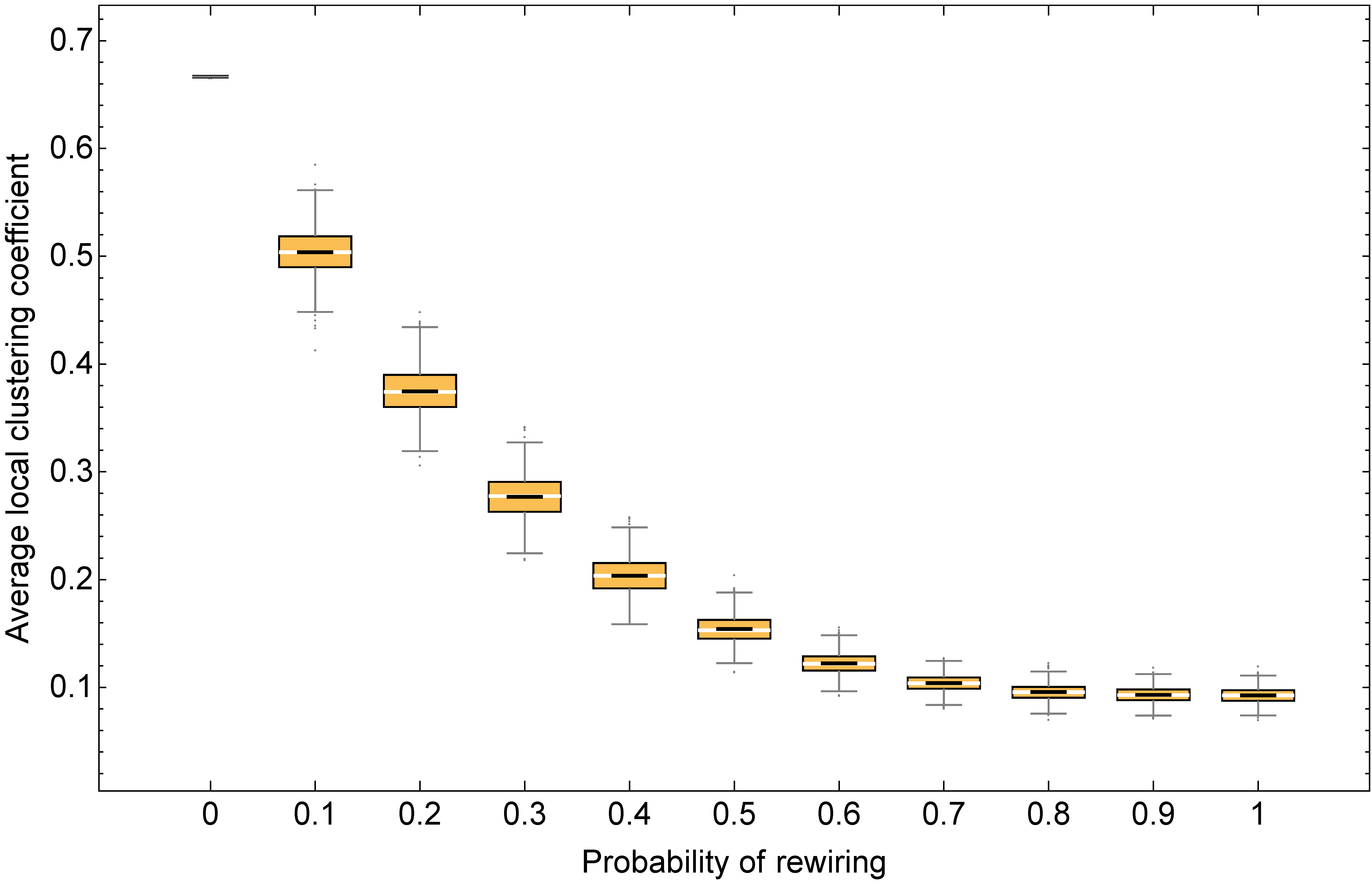
To investigate this question, the Watts–Strogatz model is very convenient, since it allows us to create networks with a fixed average degree, but with different clustering, simply by modifying the value of prob-rewiring. Figure 6 below shows several box plots of the clustering coefficient for different networks of average degree 10, obtained by running the Watts–Strogatz model with values of prob-rewiring equal to 0, 0.1, 0.2, …, 1. As you can see in figure 6, the greater the value of prob-rewiring, the lower the clustering.
Our goal now is to investigate whether clustering favors approaching the efficient state in networks of average degree 10 under our baseline conditions (i.e.: noise = 0.03, prob-revision = 0.1, and initial strategy distribution [70 30]). For that, we can run a computational experiment on Watts–Strogatz networks like the ones shown in figure 6 and, for each run, record both the average local clustering coefficient and the percentage of B-strategists by tick 5000.
Try to set up this experiment by yourself. You can find our setup below.
Experiment setup
We have set up the following experiment in BehaviorSpace:
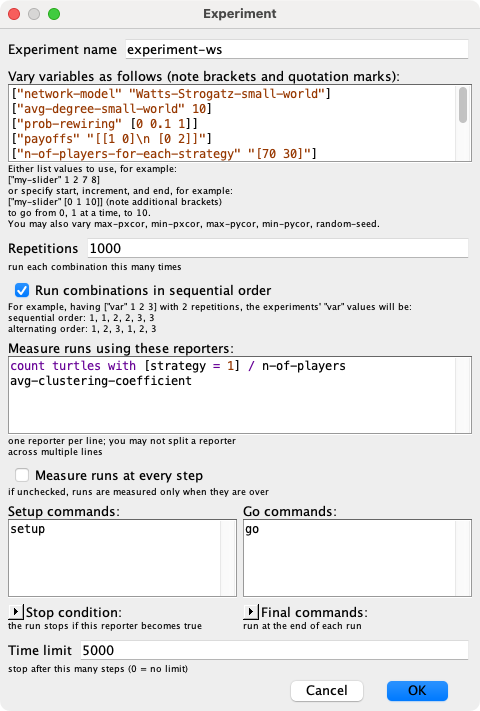
The full setting of variables for this experiment is:
["network-model" "Watts-Strogatz-small-world"]
["avg-degree-small-world" 10]
["prob-rewiring" [0 0.1 1]]
["payoffs" "[[1 0]\n [0 2]]"]
["n-of-players-for-each-strategy" "[70 30]"]
["prob-revision" 0.1]
["noise" 0.03]
["prob-link" 0.1]
["min-degree" 5]
["link-radius" 1]
We ran this experiment and, looking at the data, it was clear that –at tick 5000– most simulations were at one of two possible regimes: an inefficient one, where very few players (≤ 5%) were B-strategists, and an efficient regime, where most players (≥ 95%) were B-strategists. Thus, we decided to compute the fraction of runs in each of these two regimes, and also the fraction of those runs in none of the two regimes.[6] These fractions are shown in the following table, for different values of the (rounded) average local clustering coefficient, together with the standard errors (in brackets):[7]
| Rounded average local clustering coefficient | Total number of runs | Percentage of runs where the percentage of B-strategists is no more than 5% (inefficient regime) | Percentage of runs where the percentage of B-strategists is in the range (5%, 95%) | Percentage of runs where the percentage of B-strategists is no less than 95% (efficient regime) |
|---|---|---|---|---|
| 0.1 | 5380 | 84.14% (0.50%) | 1.64% (0.17%) | 14.22% (0.48%) |
| 0.2 | 1710 | 79.36% (0.98%) | 1.81% (0.32%) | 18.83% (0.95%) |
| 0.3 | 1037 | 69.33% (1.43%) | 2.12% (0.45%) | 28.54% (1.40%) |
| 0.4 | 879 | 53.58% (1.68%) | 2.84% (0.56%) | 43.57% (1.67%) |
| 0.5 | 980 | 26.73% (1.41%) | 1.53% (0.39%) | 71.73% (1.44%) |
| 0.6 | 14 | 14.29% (9.71%) | 0.00% (0.00%) | 85.71% (9.71%) |
| 0.7 | 1000 | 7.00% (0.81%) | 1.90% (0.43%) | 91.10% (0.90%) |
Table 1. Results of a computational experiment of our model run on Watts–Strogatz networks of avg-degree-small-world = 10 and values of prob-rewiring equal to 0, 0.1, 0.2, …, 1. Baseline conditions: noise = 0.03, prob-revision = 0.1, and initial strategy distribution [70 30]
The main insights from the data shown in table 1 above are summarized in figure 7 below.
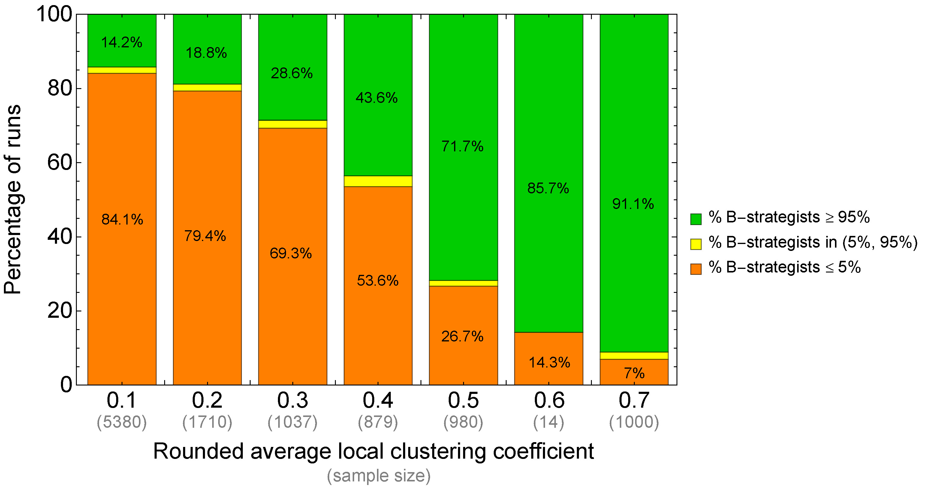
Looking at figure 7 it is clear that, as suspected, a higher clustering coefficient seems to increase the likelihood of approaching the efficient regime. However, note that this experiment has only explored networks obtained with the Watts–Strogatz model, so we do not really know whether this relation holds for other network models.
To investigate whether similar results hold for other networks, we run the same experiment as before, but with Erdős–Rényi networks and preferential attachment networks. The clustering coefficient obtained in 1000 networks created with each of these models are shown in figure 8 below:
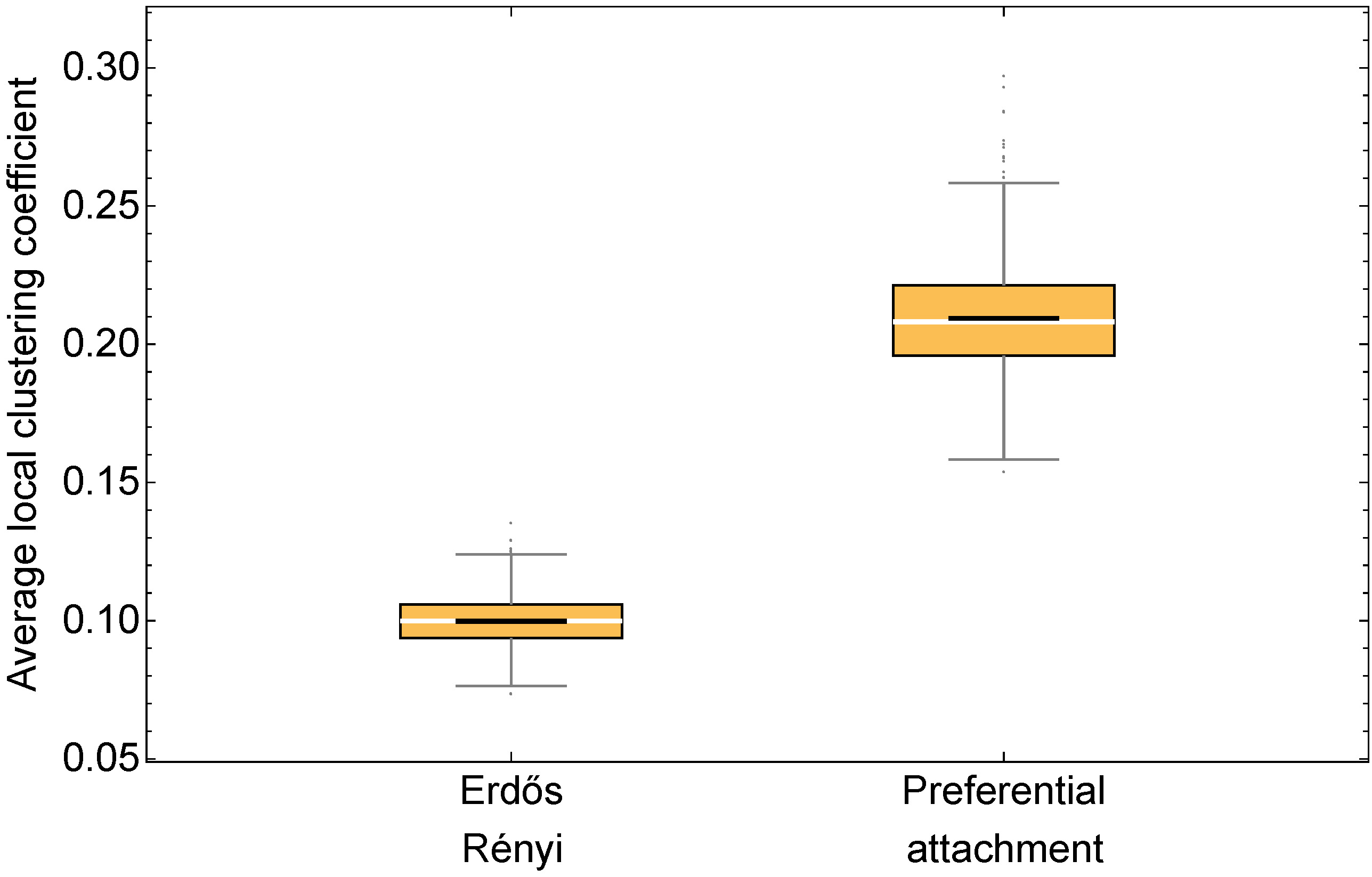
The rounded average local clustering coefficient of every Erdős–Rényi network in figure 8 is 0.1, while this value is 0.2 for 970 of the 1000 preferential-attachment networks and 0.3 for the other 30. Let us now see the proportion of runs at each of the regimes (standard errors in brackets):
| Network model | Rounded average local clustering coefficient | Total number of runs | Percentage of runs where the percentage of B-strategists is no more than 5% (inefficient regime) | Percentage of runs where the percentage of B-strategists is in the range (5%, 95%) | Percentage of runs where the percentage of B-strategists is no less than 95% (efficient regime) |
|---|---|---|---|---|---|
| Erdős–Rényi | 0.1 | 1000 | 82.20% (1.21%) | 1.50% (0.38%) | 16.30% (1.17%) |
| Preferential attachment | 0.2 | 970 | 81.96% (1.24%) | 2.37% (0.49%) | 15.67% (1.17%) |
| Preferential attachment | 0.3 | 30 | 73.33% (8.21%) | 0.00% (0.00%) | 26.67% (8.21%) |
Table 2. Results of a computational experiment of our model run on 1000 Erdős–Rényi networks with prob-link = 0.1 and 1000 preferential attachment networks with min-degree = 5. Baseline conditions: noise = 0.03, prob-revision = 0.1, and initial strategy distribution [70 30]
The main insights from the data shown in table 2 above are summarized in figure 9 below.
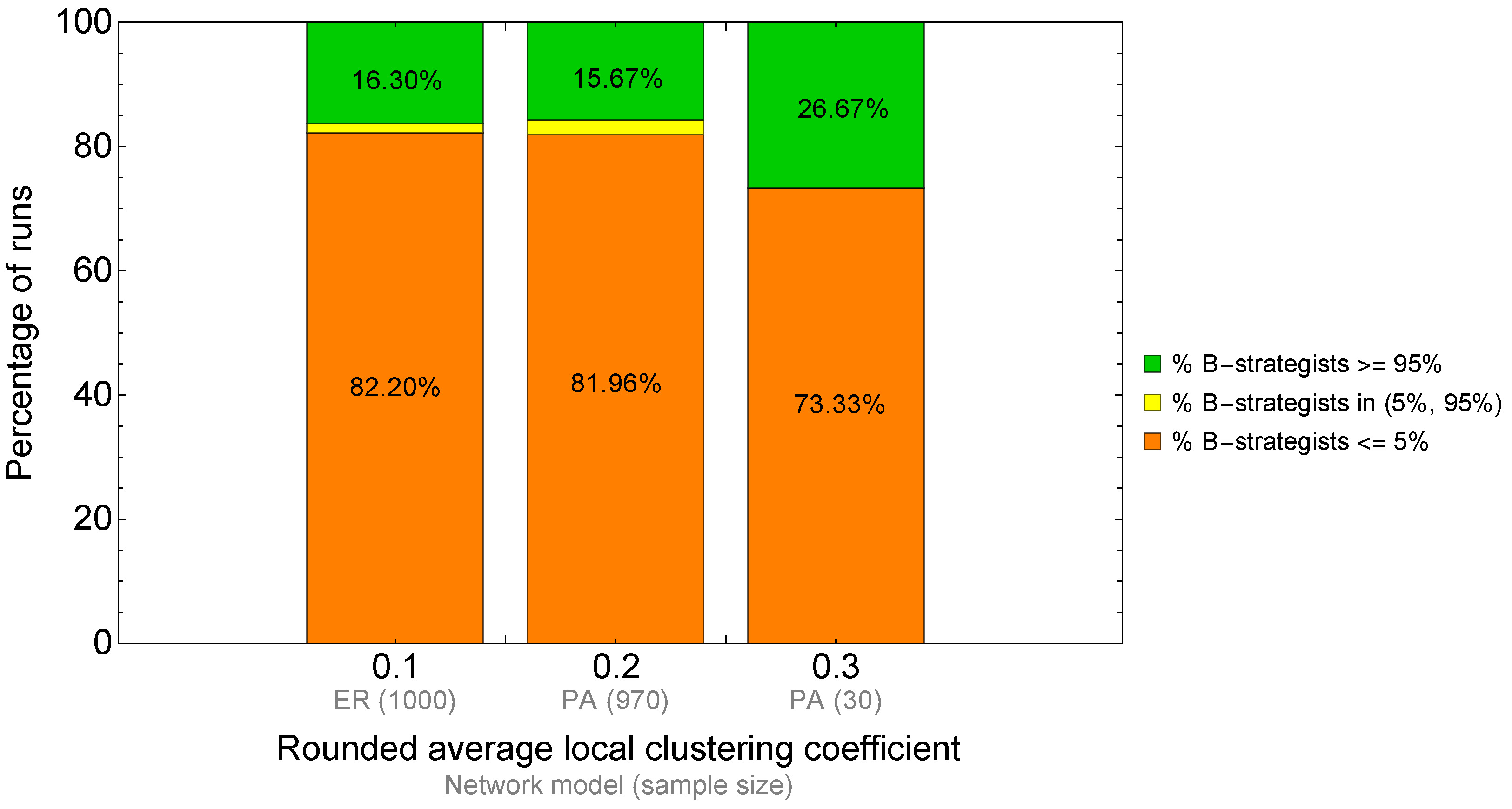
Comparing figure 7 and figure 9, it seems that the results obtained for Watts–Strogatz networks apply reasonably well to Erdős–Rényi networks and preferential attachment networks too. However, it is important not to draw conclusions beyond these network models. It is not difficult to design networks where the effect of clustering differs significantly from that observed in the network models above. The following two examples illustrate this observation.
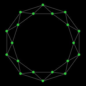
Let us start with a network with low clustering but with a high proportion of runs at the efficient regime by tick 5000. Consider the following method to build a (regular) undirected network: place the nodes in a circle, and link every node to its 10 closest spatial neighbors, after having ignored the four closest ones (i.e. ignore the two closest nodes at each side). The links of node 0 in this network are illustrated in figure 10. This network is similar to a ring lattice, but there is a gap of two nodes at either side of every node. Thus, we call this network a gap-2 ring lattice of degree 10.

The local clustering coefficient of every node in this network is ![]() . Thus, if this was a Watts–Strogatz network or a preferential attachment network, we would expect that approximately 80% of the runs would be at the inefficient regime by tick 5000 (see figure 7 and figure 9). However, we have run a 1000-run experiment to assess this, and the actual proportion of runs at the inefficient regime by tick 5000 in this type of network is only approximately 35%. It is more likely to reach the efficient regime (about 63% of the runs do it), even though the clustering coefficient is only 0.2.
. Thus, if this was a Watts–Strogatz network or a preferential attachment network, we would expect that approximately 80% of the runs would be at the inefficient regime by tick 5000 (see figure 7 and figure 9). However, we have run a 1000-run experiment to assess this, and the actual proportion of runs at the inefficient regime by tick 5000 in this type of network is only approximately 35%. It is more likely to reach the efficient regime (about 63% of the runs do it), even though the clustering coefficient is only 0.2.
Our second example illustrates the other extreme: a network with high clustering coefficient but with a low proportion of runs at the efficient regime by tick 5000. For this, we built a complete network with 27 nodes, and then we added 73 nodes; each of the new 73 nodes links to two random nodes within the set of the 27 original nodes (see figure 11).
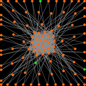
The average degree of this network is ![]() , and the average local clustering coefficient was greater than 0.9 in all the networks created for our 1000-run experiment. With such a high clustering coefficient, one would expect that more than 90% of the runs would approach the efficient regime (see figure 7). However, in our 1000-run experiment, only 23.20% of the runs were at the efficient regime by tick 5000 (and 74.70% were at the inefficient regime).
, and the average local clustering coefficient was greater than 0.9 in all the networks created for our 1000-run experiment. With such a high clustering coefficient, one would expect that more than 90% of the runs would approach the efficient regime (see figure 7). However, in our 1000-run experiment, only 23.20% of the runs were at the efficient regime by tick 5000 (and 74.70% were at the inefficient regime).
To conclude, it is important to realize that each network model implies a probability distribution over a set of networks, and the mass of this probability distribution is often concentrated on a very small proportion of networks. To put things in perspective, note that the set of all possible undirected networks with ![]() distinguishable nodes is
distinguishable nodes is ![]() . For
. For ![]() , this number is already greater than the number of protons in the observable universe (i.e. the Eddington number). When we create networks in our computers –using any model–, we are inevitably exploring a tiny proportion of all the possible networks that exist, and most often this proportion will not be representative of all the possible networks. Thus, one has to be very cautious when formulating statements about the effect of any network metric on any dynamic, if the statements are only based on simulations.
, this number is already greater than the number of protons in the observable universe (i.e. the Eddington number). When we create networks in our computers –using any model–, we are inevitably exploring a tiny proportion of all the possible networks that exist, and most often this proportion will not be representative of all the possible networks. Thus, one has to be very cautious when formulating statements about the effect of any network metric on any dynamic, if the statements are only based on simulations.
7. Exercises
You can use the following link to download the complete NetLogo model: nxn-imitate-if-better-networks-metrics.nlogo.
Exercise 1. Consider a ring lattice (i.e. the network generated with the Watts–Strogatz model using prob-rewiring = 0) where nodes have (even) degree ![]() . Assume that the number of nodes is greater than
. Assume that the number of nodes is greater than ![]() . Can you prove that every node’s local clustering coefficient is exactly
. Can you prove that every node’s local clustering coefficient is exactly ![]() ?
?
![]() Exercise 2. Can you implement a procedure to build ring lattices with arbitrary even degree without using the nw extension?
Exercise 2. Can you implement a procedure to build ring lattices with arbitrary even degree without using the nw extension?
Hint to implement a procedure to build ring lattices without using the nw extension
create-link-with player ((who + i) mod n-of-players)
![]() Exercise 3. In this chapter we defined a type of network that we named gap-2 ring lattice of degree 10 (see figure 10). Can you implement a procedure to build networks of this type with arbitrary even degree and arbitrary gap?
Exercise 3. In this chapter we defined a type of network that we named gap-2 ring lattice of degree 10 (see figure 10). Can you implement a procedure to build networks of this type with arbitrary even degree and arbitrary gap?
Exercise 4. Using the code you have created in exercise 3, run a BehaviorSpace experiment to fill in the following table for gap-x ring lattices of 100 nodes with degree 10:
| Gap | Local clustering coefficient of every node | Percentage of runs where the percentage of B-strategists is no more than 5% (inefficient regime) | Percentage of runs where the percentage of B-strategists is in the range (5%, 95%) | Percentage of runs where the percentage of B-strategists is no less than 95% (efficient regime) |
|---|---|---|---|---|
| 0 | ||||
| 1 | ||||
| 2 | ||||
| 3 | ||||
| 4 | ||||
| 5 |
![]() Exercise 5. In this chapter we built a complete network with 27 nodes. Then, we added 73 extra nodes and linked each of these new nodes to two random nodes within the set of the 27 original nodes (see figure 11). Can you implement a procedure to build this network?
Exercise 5. In this chapter we built a complete network with 27 nodes. Then, we added 73 extra nodes and linked each of these new nodes to two random nodes within the set of the 27 original nodes (see figure 11). Can you implement a procedure to build this network?
Exercise 6. Using the code you have created in exercise 5, replicate the 1000-run BehaviorSpace experiment that allowed us to say that in that network “only 23.20% of the runs were at the efficient regime by tick 5000 (and 74.70% were at the inefficient regime)”.
- By default, the local clustering coefficient is not defined for nodes with less than 2 neighbors. Here, we assume that the coefficient is 0 in those cases. ↵
- In these histograms, note that the bin for x neighbors goes from x to (x+1). For instance, in the distribution on the top left of figure 1, which corresponds to the path network, there are no nodes with degree 0, two nodes with degree 1, and 98 nodes with degree 2. ↵
- Conditions were that agents use the imitate if better rule with noise = 0.03, prob-revision = 0.1, and initial strategy distribution is 70 A-strategists and 30 B-strategists. ↵
- In Erdős–Rényi random networks, the probability that any two nodes are neighbors equals prob-link. ↵
- A simple network is one without self-links and with no more than one link between any pair of nodes. ↵
- This is something that can be easily done in an Excel spreadsheet, by defining a column for each regime, such that the value of the corresponding row equals 1 if the run is in the regime and 0 otherwise. The average of this column is the fraction of runs at the regime. ↵
- The frequency of the event "the population is at a certain regime" calculated over n simulation runs can be seen as the mean of a sample of n i.i.d. Bernouilli random variables where success denotes that the event occurred and failure denotes that it did not. Thus, the frequency f is the maximum likelihood (unbiased) estimator of the exact probability with which the event occurs. The standard error of the calculated frequency f is the standard deviation of the sample divided by the square root of the sample size. In this particular case, the formula reads:
Std. error (f, n) = (f (1 — f) / (n — 1))1/2 ↵
