
Part V. Agent-based models vs ODE models
V-3. Mean Dynamics
1. Introduction
Every dynamic that can be run with the NetLogo model we have implemented in the previous chapter (nxn-games-in-well-mixed-populations.nlogo) can be usefully seen as a time-homogeneous Markov chain on the space of possible strategy distributions. This means that the fraction of agents that are using each strategy, i.e., the population state, contains all the information we need to –probabilistically– predict the evolution of the agent-based dynamic as accurately as it is possible.
Let  denote the fraction of agents using strategy
  . In games with
  strategies, population states
  are elements of the simplex
  . More specifically, if there are
  agents, population states are elements of the finite grid
  .
.
A fully parameterized model defines a discrete-time Markov chain  on state space
  , where
  is the index for the ticks. Our goal in this chapter is to approximate the transient dynamics of this (stochastic) process with its corresponding (deterministic) mean dynamic.
In the next section, we explain how to derive the mean dynamic in general, and in section 3 we present the mean dynamic for every possible parameterization of NetLogo model nxn-games-in-well-mixed-populations.nlogo. Then, in section 4 we show how we can numerically solve the mean dynamic using the Euler method within NetLogo. In section 5, we present some representative simulations together with their corresponding mean dynamics solved at runtime within NetLogo. In this way, we will be able to appreciate how useful the mean dynamic can be. We conclude the chapter (and the book) emphasizing how sensitive agent-based evolutionary dynamics can be to seemingly unimportant details.
2. The mean dynamic
The mean dynamic (Benaïm & Weibull, 2003; Sandholm, 2010a, chapter 10; Roth & Sandholm, 2013) is a system of ODEs that provides a good deterministic approximation to the dynamics of the stochastic evolutionary process
- over finite time spans,
- when the number of agents is sufficiently large, and
- when the revision probability is sufficiently low.
To derive the mean dynamic, we consider the behavior of the process over the next  time units, departing from population state
  . For convenience, we define one unit of clock time as 1/prob-revision ticks, i.e., the number of ticks over which every agent is expected to receive exactly one revision opportunity.[1] Thus, over the time interval , the number of agents who are expected to receive a revision opportunity is
Of the  agents who revise their strategies over the time interval ,
  are expected to be
  -strategists. Let
  be the conditional probability that a reviser using strategy adopts strategy (so
  denotes the probability that a reviser using strategy keeps using strategy after revision). Using this notation, the expected number of -revisers who adopt strategy over the time interval is
  Hence, the expected change in the number of agents that are using strategy over the time interval equals:
- the number of revisers who adopt strategy , i.e. the inflow, which is
 ,
, - minus the number of -revisers, i.e. the outflow, which is
 .
.
Therefore, the expected change in the fraction of agents using strategy , i.e. the expected change in variable at population state , is:

Note that conditional probabilities may depend on . This does not represent a problem as long as this dependency vanishes as gets large. In that case, to deal with that dependency, we take the limit of as goes to infinity since, after all, the mean dynamic approximation is only valid for large . Thus, defining

we arrive at the mean dynamic equation for strategy :
 |
(1) |
An equivalent formulation that is sometimes more convenient to use is the following:
 |
(2) |
The two formulations above only differ in how they treat -revisers who keep strategy . In the first formulation (1), these agents are included both in the inflow and in the outflow, while in the second formulation (2) they are excluded from both flows. In any case, it is clear that all we need to derive the mean dynamic of a model is the conditional probabilities  .
.
Finally, introducing noise in the mean dynamic is not difficult. If noise  , i.e., if revisers choose a random strategy with probability
  , and with probability
  they adopt strategies with conditional probabilities
  , the first formulation of the general mean dynamic (1) would be:

And the second formulation would be adapted as follows:

3. Derivation of the mean dynamic for different stochastic processes
In this section we derive the mean dynamic for every possible parameterization of the NetLogo model we developed in the previous chapter (nxn-games-in-well-mixed-populations.nlogo). In particular, we analyze every possible combination of values for parameters decision-rule and payoff-to-use. For each combination of these two parameter values, we provide a formula for the mean dynamic that is valid for any game (payoffs) and any initial condition (n-of-players-for-each-strategy). The impact of noise can be easily taken into account as explained above. The mean dynamic will be a good approximation for the transient dynamics of the corresponding agent-based model when prob-revision is low and the population size is large.
3.1. Imitate if better
payoff-to-use = “play-with-one-rd-agent“
The probability that a reviser is a -player with payoff  is
is  . The probability that the observed agent is an -player with payoff
  is
is  .
.
The probability that a -player with payoff observes an -player with payoff is  .
.
Considering that the revising -player adopts the strategy of the -player if  , the total
  of -players who switch to strategy (adding for every
  ) is
) is

and the total  of -strategists who switch to some other strategy is

The mean dynamic is then

This rule has been studied by Izquierdo and Izquierdo (2013) and Loginov (2021). Loginov (2021) calls this rule “imitate-the-better-realization”.
payoff-to-use = “use-strategy-expected-payoff“
The probability that a reviser is a -player (whose payoff is  ) who observes an -player (whose payoff is
  ) is
) is  .
.
Considering that the revising -player adopts the strategy of the -player iff  , the total of -players who switch to strategy (adding for every ) is

and the of -strategists who switch to some other strategy is

The mean dynamic is then

3.2. Imitative pairwise-difference
 ) minus the minimum possible payoff (
 ).
).payoff-to-use = “play-with-one-rd-agent“
The probability that a reviser is a -player with payoff is . The probability that the observed agent is an -player with payoff is . The probability that a -player with payoff observes an -player with payoff is .
Considering that the revising -player adopts the strategy of the -player with probability ![\frac{ [\pi_{ik}-\pi_{jl}]_+}{M-m},](https://wisc.pb.unizin.org/app/uploads/quicklatex/quicklatex.com-c8e9a460a9360977b37978ba4934bc10_l3.png "Rendered by QuickLaTeX.com") the total of -players who switch to strategy (adding for every ) is[2]
the total of -players who switch to strategy (adding for every ) is[2]
![Inflow_i (x) = \sum_{j \neq i} x_j \, p^\infty_{ji}(x) = \sum_{j \neq i} x_j x_i \sum_k x_k \sum_{l} x_l \frac{ [\pi_{ik}-\pi_{jl}]_+}{M-m}](https://wisc.pb.unizin.org/app/uploads/quicklatex/quicklatex.com-e3b42674a487949fcc5ebcc5d1d59be8_l3.png "Rendered by QuickLaTeX.com")
and the of -strategists who switch to some other strategy is
![Outflow_i (x) = x_i \sum_{j \neq i} p^\infty_{ij}(x) = x_i \sum_{j \neq i} x_j \sum_k x_k \sum_l x_l \frac{ [\pi_{jl} - \pi_{ik}]_+}{M-m}](https://wisc.pb.unizin.org/app/uploads/quicklatex/quicklatex.com-a5051460dd83add4f726fbd394dc7cd7_l3.png "Rendered by QuickLaTeX.com")
The mean dynamic is then
![\begin{align*} \dot{x}_i &= Inflow_i (x) - Outflow_i (x) \\ &= \frac{x_i}{M-m} \sum_{j \neq i} x_j \sum_k x_k \sum_{l} x_l \left([\pi_{ik}-\pi_{jl}]_+ - [\pi_{jl} - \pi_{ik}]_+ \right) \\ &= \frac{x_i}{M-m} \sum_{j \neq i} x_j \sum_k x_k \sum_{l} x_l (\pi_{ik}-\pi_{jl}) \\ &= \frac{x_i}{M-m} (\pi_i - \pi)\end{align*}](https://wisc.pb.unizin.org/app/uploads/quicklatex/quicklatex.com-c7821e973c8855c2908524772161c4b7_l3.png "Rendered by QuickLaTeX.com")
This ODE is the replicator dynamics with a constant speed factor  The orbits of the mean dynamic do not change with the speed factor. However, if we are interested in the relationship between the solution of the mean dynamic at a given time
  and the stochastic process after a number of ticks, then the speed factor must be considered.
payoff-to-use = “use-strategy-expected-payoff“
The probability that a revising -player (with payoff ) observes an -player (with payoff ) is .
Considering that the revising -player adopts the strategy of the -player with probability ![\frac{ [\pi_{i}-\pi_{j}]_+}{M-m}](https://wisc.pb.unizin.org/app/uploads/quicklatex/quicklatex.com-02f3de6180b2cbb48eb12ced44ca2c45_l3.png "Rendered by QuickLaTeX.com") , the total of -players who switch to strategy (adding for every ) is
, the total of -players who switch to strategy (adding for every ) is
![Inflow_i (x) = \sum_{j \neq i} x_j \, p^\infty_{ji}(x) = \sum_{j \neq i} x_j x_i \frac{ [\pi_{i}-\pi_{j}]_+}{M-m}](https://wisc.pb.unizin.org/app/uploads/quicklatex/quicklatex.com-c061efc767f6e26ba84938d0241b5611_l3.png "Rendered by QuickLaTeX.com")
and the of -strategists who switch to some other strategy is
![Outflow_i (x) = x_i \sum_{j \neq i} p^\infty_{ij}(x) = x_i \sum_{j \neq i} x_j \frac{ [\pi_{j} - \pi_{i}]_+}{M-m}](https://wisc.pb.unizin.org/app/uploads/quicklatex/quicklatex.com-3532705da5de0339ce8575f1df3d5d46_l3.png "Rendered by QuickLaTeX.com")
The mean dynamic is then
![\begin{align*} \dot{x}_i &= Inflow_i (x) - Outflow_i (x) \\ &= \frac{x_i}{M-m} \sum_{j \neq i} x_j \left([\pi_{i}-\pi_{j}]_+ - [\pi_{j} - \pi_{i}]_+ \right)\\ &= \frac{x_i}{M-m} \sum_{j \neq i} x_j (\pi_{i}-\pi_{j}) \\ &= \frac{x_i}{M-m} (\pi_i - \pi)\end{align*}](https://wisc.pb.unizin.org/app/uploads/quicklatex/quicklatex.com-85ec1ee775677d6ccb512f301425ea7a_l3.png "Rendered by QuickLaTeX.com")
This ODE is the replicator dynamics with constant speed factor  .
.
3.3. Imitative linear attraction
), divided by the maximum possible payoff () minus the minimum possible payoff. (The revising agent’s payoff is ignored.)payoff-to-use = “play-with-one-rd-agent“
The probability that a revising -player observes an -player with payoff is  .
.
Considering that the revising -player adopts the strategy of the -player with probability  , the total of -players who switch to strategy (adding for every ) is

and the of -strategists who switch to some other strategy is

The mean dynamic is then

This ODE is the replicator dynamics with constant speed factor .
payoff-to-use = “use-strategy-expected-payoff“
The probability that a revising -player observes an -player (whose payoff is ) is .
Considering that the revising -player adopts the strategy of the -player with probability  , the total of -players who switch to strategy (adding for every ) is

and the of -strategists who switch to some other strategy is

The mean dynamic is then

This ODE is the replicator dynamics with constant speed factor .
3.4. Imitative linear dissatisfaction
) and his own payoff, divided by the maximum possible payoff minus the minimum possible payoff (). (The observed agent’s payoff is ignored.)payoff-to-use = “play-with-one-rd-agent“
The probability that a revising -player with payoff  observes an -player is
  .
.
Considering that the revising -player adopts the strategy of the -player with probability  , the total of -players who switch to strategy (adding for every ) is

and the of -strategists who switch to some other strategy is

The mean dynamic is then

Again, this ODE is the replicator dynamics with constant speed factor .
payoff-to-use = “use-strategy-expected-payoff“
The probability that a revising -player (whose payoff is ) observes an -player is .
Considering that the revising -player adopts the strategy of the -player with probability  , the total of -players who switch to strategy (adding for every ) is

and the of -strategists who switch to some other strategy is

The mean dynamic is then

Again, this ODE is the replicator dynamics with constant speed factor .
3.5. Direct best
payoff-to-use = “play-with-one-rd-agent“
Under this process, a revising agents tests each of the possible strategies once (with each play of each strategy being against a newly drawn opponent) and selects one of the strategies that obtained the greatest experienced payoff in the test. Ties are resolved uniformly at random, with equal probability for each of the maximum-payoff strategies.
Note that which strategy is selected depends on what strategy is sampled (i.e., which strategy is used by the sampled co-player) when testing each of the strategies, and we will need some notation to refer to the strategy  of the agent that is sampled when testing strategy . Consider the following notation:
- Sample list
 . Considering a sample of agents (one for each tested strategy), let a sample list
  be a list whose -th component indicates the strategy of the agent that was sampled when testing strategy . Let
  be the set of all such lists of strategies of length . For instance,
  , with e.g. sample list (2,1) indicating that when testing strategy 1 (first position) the sampled agent (co-player) played strategy 2 (element in first position), and when testing strategy 2 (second position) the sampled agent played strategy 1 (element in position 2).
  : probability of obtaining sample list at state . This probability is
  .
.- Experienced payoff vector
 . This is the vector of experienced payoffs obtained by testing each of the strategies, when the strategies of the sampled co-players are those in . The -th component of this payoff vector,
  , is the payoff to an agent testing strategy whose co-player uses strategy .
 - Best experienced payoff indicator for strategy ,
 . Given an experienced payoff vector , this function returns the value 1 if strategy obtains the maximum payoff in , i.e., if
  , and the value 0 otherwise.
With the previous notation, adding the probabilities of all the events that lead a revising agent to choose strategy , we have

 is given by the fraction of revisers that are -players, i.e.,
  .
.
The mean dynamic is then

This is a best-experienced-payoff dynamic analyzed by Osborne and Rubinstein (1998), Sethi (2000, 2021) and Sandholm et al. (2019, 2020).
payoff-to-use = “use-strategy-expected-payoff“
Under this process, a revising agent adopts one of the strategies with the greatest expected payoff in the population. This is a best-response dynamic. The greatest expected payoff obtained by (one or several) strategies at state is  . Let
. Let  be the set of stategies that obtain the greatest expected payoff
  at state and let
  be the cardinality of that set, i.e., the number of strategies that obtain the maximum expected payoff at state .
The probability that a reviser adopts strategy is then

is given by the fraction of revisers that are -players, i.e., . Thus, the mean dynamic is

Gilboa and Matsui (1991), Hofbauer (1995b) and Kandori and Rob (1995) are pioneering references on best-response dynamics.
3.6. Direct pairwise-difference
minus the minimum possible payoff .payoff-to-use = “play-with-one-rd-agent“
The probability that the revising agent is a -player with payoff and he selects candidate strategy , with a payoff  obtained for strategy , is
  .
.
Considering that the revising -player adopts the strategy of the -player with probability ![\frac{ [\pi_{il}-\pi_{jk}]_+}{M-m},](https://wisc.pb.unizin.org/app/uploads/quicklatex/quicklatex.com-9e541af4c2db4a33f1b19ca8cf93e1b1_l3.png "Rendered by QuickLaTeX.com") the total of -players who switch to strategy (adding for every ) is
the total of -players who switch to strategy (adding for every ) is
![Inflow_i (x) = \frac{1}{(n-1)(M-m)} \sum_{j \neq i,k,l} x_j x_k x_l [\pi_{il}-\pi_{jk}]_+](https://wisc.pb.unizin.org/app/uploads/quicklatex/quicklatex.com-585ec5213147605c3c6877bd6e623c85_l3.png "Rendered by QuickLaTeX.com")
and the of -strategists who switch to some other strategy is
![Outflow_i (x) = x_i \frac{1}{(n-1)(M-m)} \sum_{j \neq i,k,l} x_k x_l [\pi_{jk} - \pi_{il}]_+](https://wisc.pb.unizin.org/app/uploads/quicklatex/quicklatex.com-755499801453e31b5ff76d2f2971bc7c_l3.png "Rendered by QuickLaTeX.com")
The mean dynamic is then
![\begin{align*} \dot{x}_i &= Inflow_i (x) - Outflow_i (x) \\ &= \frac{1}{(n-1)(M-m)} \sum_{j \ne i} \left(x_j \sum_{k,l} x_k \, x_l [\pi_{il}-\pi_{jk}]_+ - x_i \sum_{k,l} x_k \, x_l [\pi_{jk} - \pi_{il}]_+\right) \\ \end{align*}](https://wisc.pb.unizin.org/app/uploads/quicklatex/quicklatex.com-305a0685e5dab0f08a93b5739896fc36_l3.png "Rendered by QuickLaTeX.com")
payoff-to-use = “use-strategy-expected-payoff“
The probability that the revising agent is a -player (with payoff ) and he selects candidate strategy (with payoff ) is  .
.
Considering that the revising -player adopts the strategy of the -player with probability ![\frac{ [\pi_{i}-\pi_{j}]_+}{M-m},](https://wisc.pb.unizin.org/app/uploads/quicklatex/quicklatex.com-bfe24a660efd6c45c167aa7085f13441_l3.png "Rendered by QuickLaTeX.com") the total of -players who switch to strategy (adding for every ) is
the total of -players who switch to strategy (adding for every ) is
![Inflow_i (x) = \frac{1}{(n-1)(M-m)} \sum_{j \neq i} x_j [\pi_{i}-\pi_{j}]_+](https://wisc.pb.unizin.org/app/uploads/quicklatex/quicklatex.com-428584a09349d69d2daf74415f69ff3b_l3.png "Rendered by QuickLaTeX.com")
and the of -strategists who switch to some other strategy is
![Outflow_i (x) = x_i \frac{1}{(n-1)(M-m)} \sum_{j \neq i} [\pi_{j} - \pi_{i}]_+](https://wisc.pb.unizin.org/app/uploads/quicklatex/quicklatex.com-6baab3f1eaaa18011ced84a90963c12b_l3.png "Rendered by QuickLaTeX.com")
The mean dynamic is then
![\begin{align*} \dot{x}_i &= Inflow_i (x) - Outflow_i (x) \\ &= \frac{1}{(n-1)(M-m)} \sum_{j} \left(x_j [\pi_{i}-\pi_{j}]_+ - x_i [\pi_{j} - \pi_{i}]_+\right) \\ \end{align*}](https://wisc.pb.unizin.org/app/uploads/quicklatex/quicklatex.com-26fe5f4fb8a7dc6e80d995604aadb779_l3.png "Rendered by QuickLaTeX.com")
This is the Smith dynamic (Smith, 1984; Sandholm, 2010b) with constant speed factor  .
.
3.7. Direct positive proportional
payoff-to-use = “play-with-one-rd-agent“
Under this process, using the notation introduced for decision rule “direct-best“, the probability that a reviser selects strategy is

is given by the fraction of revisers that are -players, i.e., .
The mean dynamic is then

payoff-to-use = “use-strategy-expected-payoff“
Under this process, the probability that a reviser selects strategy is

is given by the fraction of revisers that are -players, i.e., .
The mean dynamic is then

4. Running an agent-based model and solving its mean dynamic at runtime
In this section, we explain the Euler method to solve ODEs and we show how to implement it in NetLogo. For illustration purposes we use the 1-2 coordination game, which is the 2-player 2-strategy single-optimum coordination game that we introduced in chapter I-2 and analyzed in Part IV. Its payoff matrix is shown in Figure 1 below:
| Player 2 | |||
| Player 2 chooses A | Player 2 chooses B | ||
| Player 1 | Player 1 chooses A | 1 , 1 | 0 , 0 |
| Player 1 chooses B | 0 , 0 | 2 , 2 | |
Figure 1. Payoffs for the 1-2 coordination game
4.1. The Euler method to numerically solve ODEs
Since there are only two strategies in the 1-2 coordination game, the mean dynamic can be expressed using one single variable. Let denote the fraction of B-strategists.
To solve the mean dynamic, we use the Euler method, which is one of the simplest numerical procedures for solving ODEs with an initial condition. Consider the ODE  with initial condition
  Our goal is to compute a series of values
  which will approximate the solution trajectory
  that departs from initial value
  . Note that in this section
  denotes a value in the series (not the fraction of -strategists).
We start by setting  , i.e. the first point in our series is the initial condition. To compute the following values
  we proceed recursively as follows:

where  is a step size chosen by us.
Geometrically, note that  can be interpreted as the slope of the tangent line to the solution curve at
  . So basically, departing from , we are approximating the value of the solution trajectory after time units using the tangent line at , which is the best linear approximation to the curve at that point (see Figure 2 below).
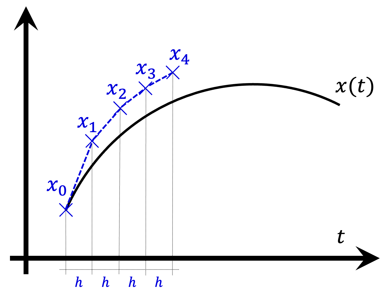
In this way, by using the Euler method, we are approximating the solution curve with initial value by the series of line segments that connect the consecutive points . The value is the approximation to the solution curve with initial value after  time units.
How should we choose the value of step size ? In general, the lower the value of , the better the approximation. Here, since we are going to run a discrete-time simulation and solve its mean dynamic at the same time, a natural candidate is to choose the time that corresponds to one tick in the NetLogo model. And how long is that? Recall that, in section 2 above, we derived the mean dynamic defining one unit of clock time as 1/prob-revision ticks. Therefore, one tick corresponds to prob-revision time units, so we choose  prob-revision.
4.2. Solving an ODE numerically within NetLogo
As an example, consider the agent-based dynamic with decision-rule = “direct-positive-proportional-m“, m = 1, and payoff-to-use = “play-with-one-rd-agent“. The mean dynamic for this setting in the 1-2 coordination game (Fig. 1) is:

where is the number of B-strategists.
Therefore, using the Euler method we compute the value  from as follows:

In NetLogo, we can define a global variable x and we can update its value every tick as follows:
set x x + prob-revision * x * (1 - x) / 6
For simplicity, here we have discussed a model where the mean dynamic has one single independent variable, but the Euler method can be used (and implemented within NetLogo) with any number of variables.[3]
4.3. The influence of population size
Figure 3 below shows some representative simulations of the parameterization considered in the previous section for different population sizes. The numerical solution of the mean dynamic  is shown as a black line in every plot. All these graphs have been created with NetLogo model nxn-games-in-well-mixed-populations-md.nlogo, which numerically solves the mean dynamic for any setting in the 1-2 coordination game, at runtime.
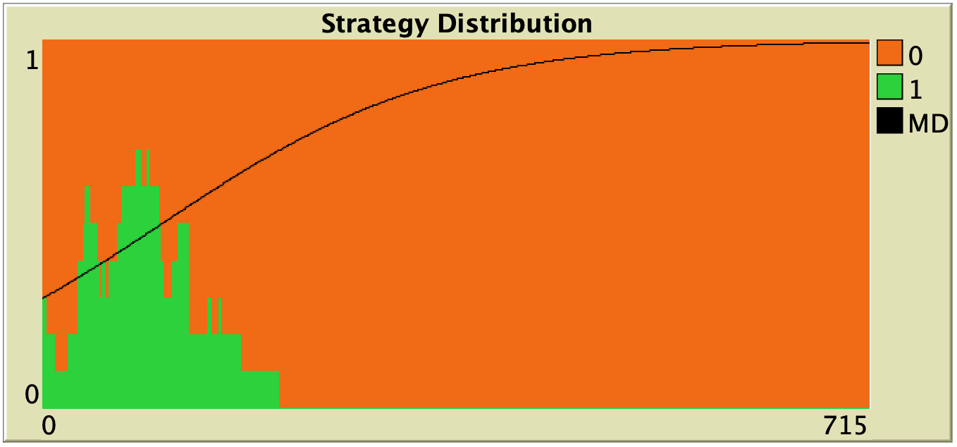
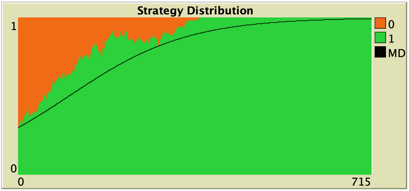
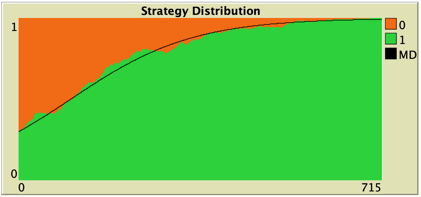
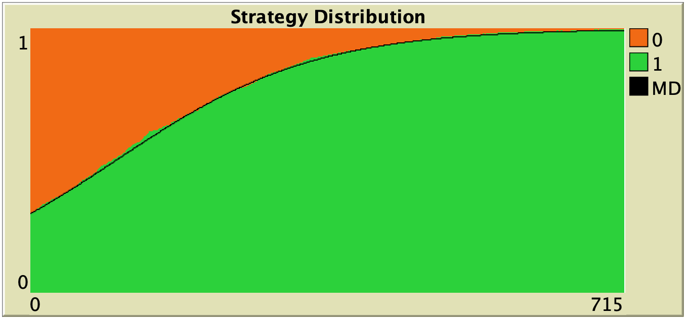
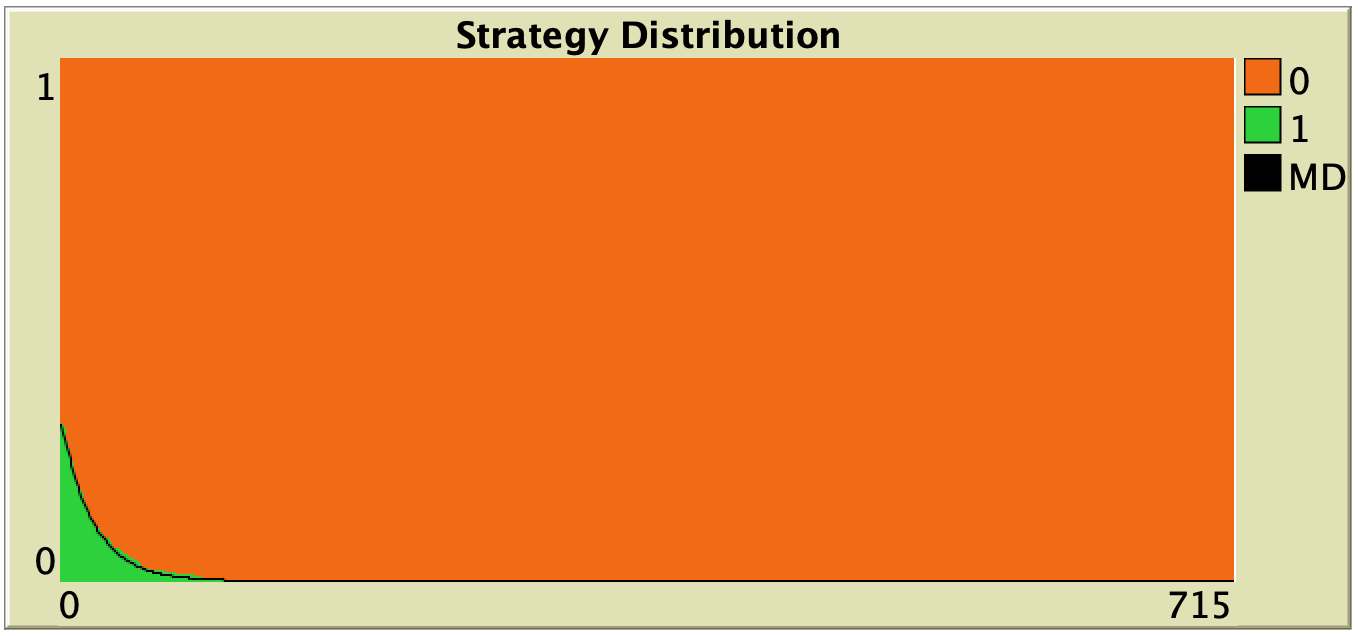
Figure 3. Representative simulation runs executed with NetLogo model nxn-games-in-well-mixed-populations-md.nlogo, for different population sizes . The black line shows the numerical solution of the mean dynamic, obtained using the Euler method. Settings are: decision-rule = “direct-positive-proportional-m“, m = 1, payoff-to-use = “play-with-one-rd-agent“, noise = 0 and prob-revision = 0.05. The game is the 1-2 coordination game. Initially, 70% of the agents are A-strategists (orange) and 30% are B-strategists (green)
As you can see in Figure 3, the greater the population size , the better the mean dynamic approximates the stochastic dynamics of our agent-based model. As grows, the stochastic fluctuations of the agent-based model (in strategy proportions) diminish, and simulations tend to get closer and closer to the –deterministic– solution of the mean dynamic.
5. Representative simulations together with their mean dynamics
In this section we explore the influence of parameters decision-rule and payoff-to-use in our model. Table 1 below shows representative simulations for different values of these parameters in the 1-2 coordination game, including the numerical solution of the corresponding mean dynamic as a black line. All these graphs can be replicated using NetLogo model nxn-games-in-well-mixed-populations-md.nlogo. The equation displayed under each plot is the corresponding mean dynamic (where denotes the fraction of B-strategists, which is shown in green in the plots).
| decision-rule | payoff-to-use | |
|---|---|---|
| play-with-one-rd-agent | use-strategy-expected-payoff | |
| Imitate if better | 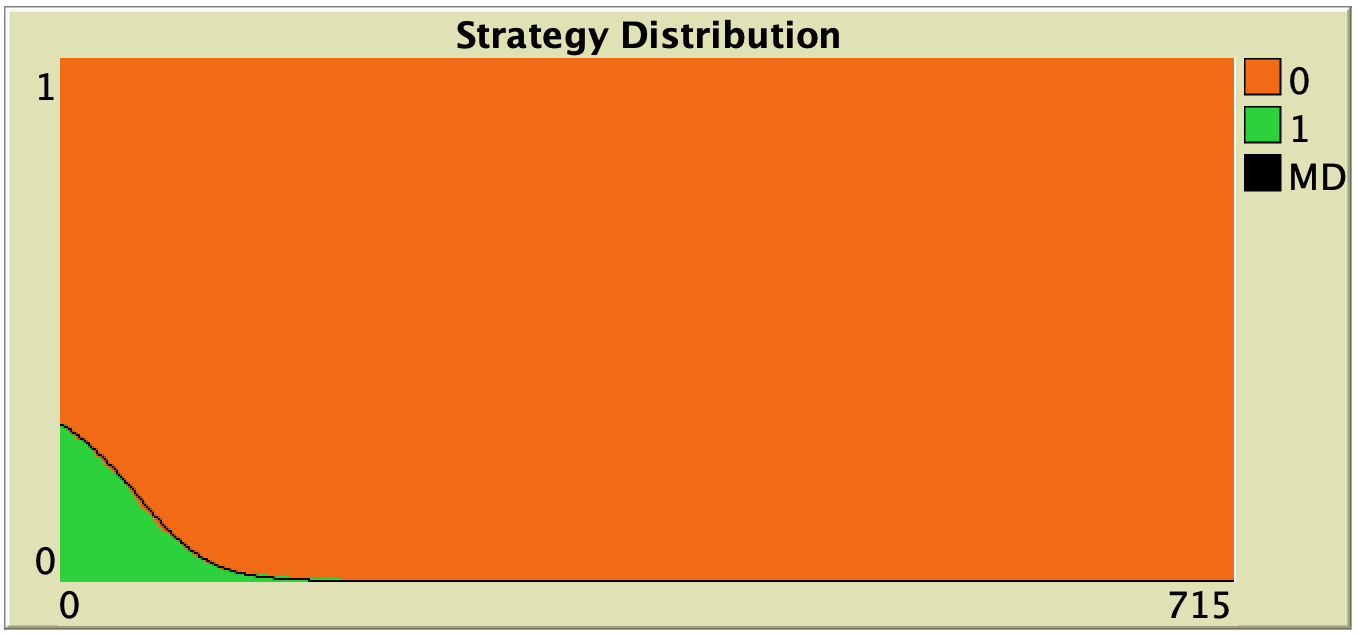 |
 |
 |
 |
|
| Imitative pairwise-difference | 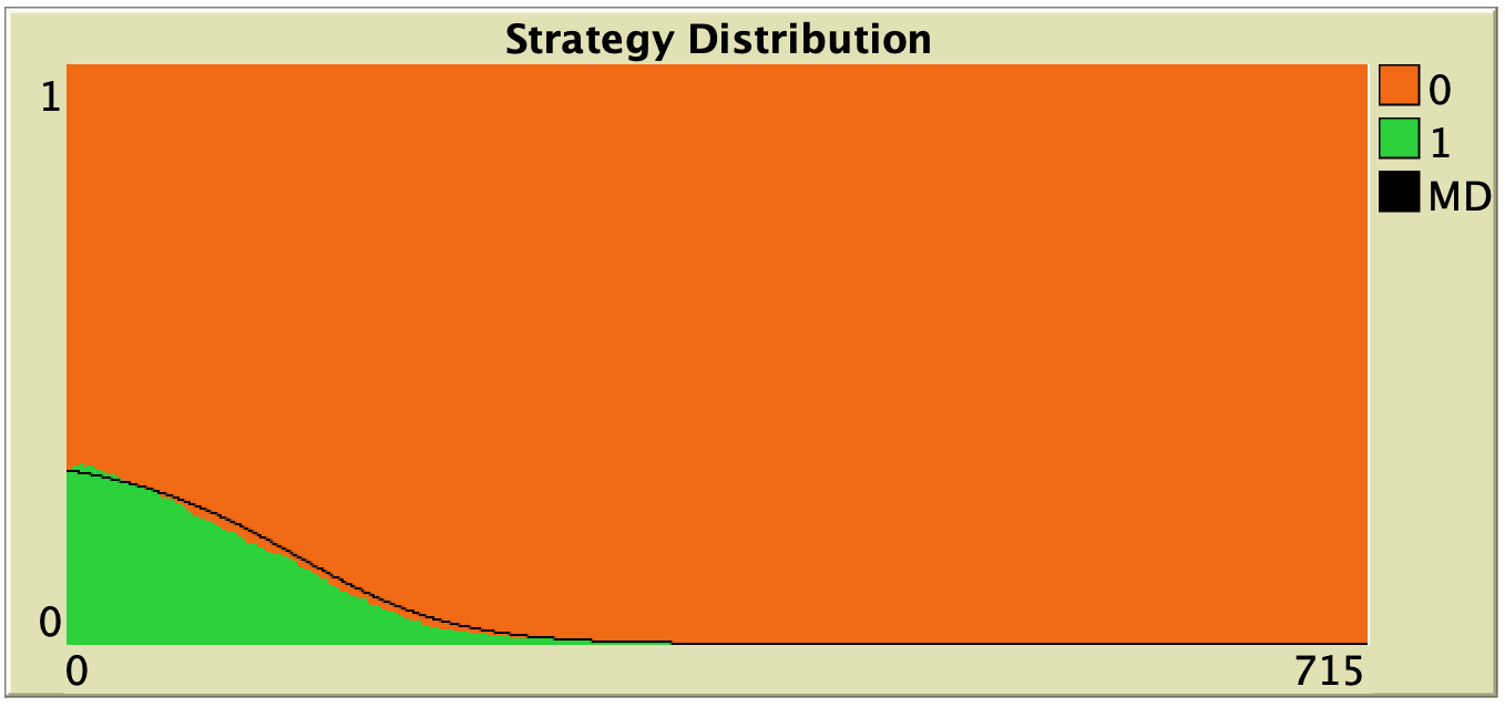 |
 |
 |
|
|
| Direct best | 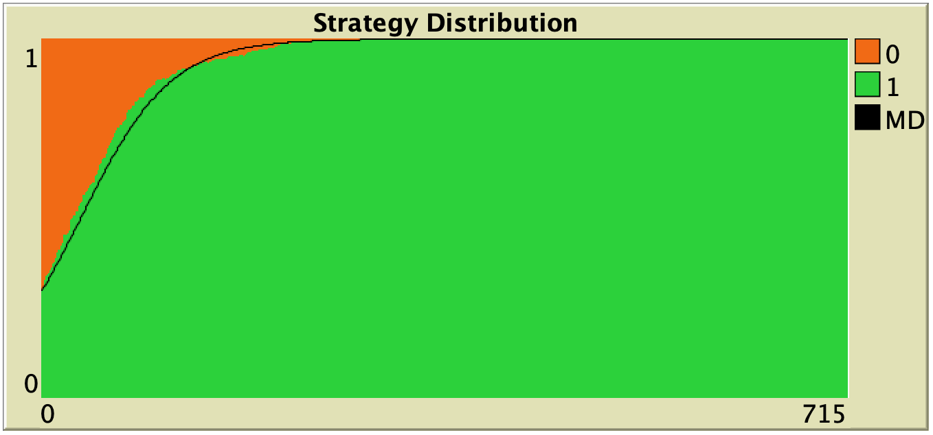 |
 |
 |
 |
|
| Direct pairwise-difference | 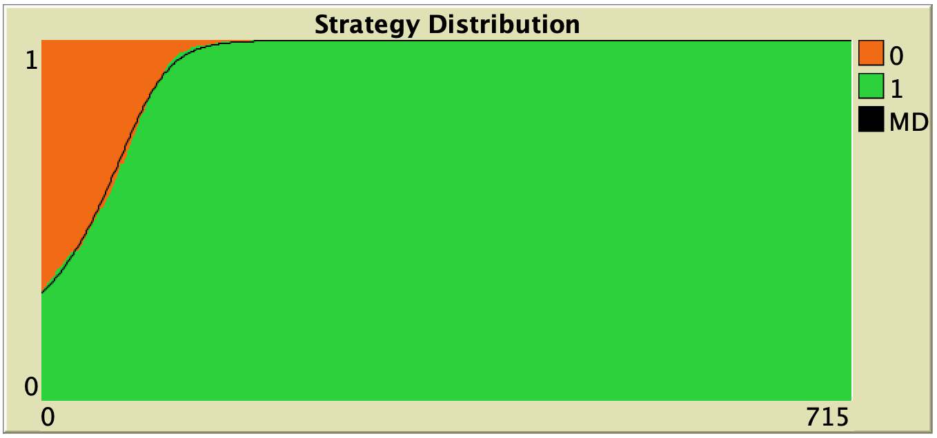 |
 |
 |
 |
|
| Direct positive proportional m = 1 |
|
 |
 |
 |
|
| Direct positive proportional m = 10 |
 |
 |
|
|
|
Table 1. Representative simulation runs executed with NetLogo model nxn-games-in-well-mixed-populations-md.nlogo, for different decision rules and different ways of computing payoffs. Initial conditions are [700 300], i.e. 700 A-strategists (in orange) and 300 B-strategist (in green), prob-revision = 0.05 and there is no noise. The equation of the mean dynamic (where denotes the fraction of B-strategists) is included under each plot. The black line shows the numerical solution of the mean dynamic, obtained using the Euler method
The results shown in Table 1 allow us to draw a number of observations. The most obvious one is that the mean dynamic provides a very good approximation for the dynamics of all parameterizations shown in the table. The population size in all simulations shown in Table 1 is  . The approximation would become even better for greater population sizes (and would degrade for lower population sizes).
Looking at Table 1, it is also clear that we can make the population go to one monomorphic state or the other simply by changing the value of parameter decision-rule and, in some cases, the value of payoff-to-use. These two parameters affect the dynamics in ways that do not seem easy to understand without the help of the mean dynamic.
Finally, in terms of mean dynamics, note that only one of the rows in Table 1 corresponds to the replicator dynamics (i.e., the row for decision-rule = “imitative-pairwise-difference“).[4] The other decision rules in Table 1 have mean dynamics that are different from the replicator dynamics; and, in many cases, these other dynamics lead to the opposite end of the state space. For this reason, it seems clear that we should not make general statements about evolutionary dynamics if such statements are based only on the behavior of the replicator dynamics (or any other particular model, for that matter). There are many other evolutionary dynamics that lead to results completely different from those obtained with the replicator dynamics.
To be clear, in our view, all the decision rules in Table 1 could be defended as sensible models of evolution in the sense that, under all of them, agents preferentially switch to strategies that provide greater payoffs. Nonetheless, they lead to completely different dynamics. It is true that the replicator dynamics appears as the mean dynamic of many different agent-based models (see chapter V-1), but it is also true that there are a myriad of other sensible models of evolution with properties completely different from those of the replicator dynamics.
6. Details matter
In previous chapters of this book, we learned that evolutionary dynamics on grids (and, more generally, on networks) can be significantly affected by small, seemingly unimportant details. In this final chapter, we have seen that this sensitivity to apparently innocuous details can also be present in the simpler setting of well-mixed populations. In general, evolutionary game dynamics in well-mixed populations can also depend on factors that may seem insignificant at first sight. Because of this, if we had to summarize this book in one sentence, this sentence could well be: “Details matter”
This sensitivity to small details suggests that a simple general theory on evolutionary game dynamics cannot be derived. It also highlights the usefulness of the skills you have acquired with this book. We hope that you have learned new ways to explore and tame the complexity and the beauty of evolutionary game dynamics, using both computer simulation and mathematical analysis.
7. Exercises

Exercise 1. Derive the mean dynamic for a decision rule that you can call “imitate-the-best” using expected payoffs (Hofbauer, 1995a; Vega-Redondo, 1997). Under this rule, the revising agent copies the strategy of the individual with the greatest expected payoff. Resolve ties uniformly at random.
Exercise 2. Derive the mean dynamic for a decision rule that you can call “imitative-positive-proportional” assuming agents obtain their payoff by playing with one random agent, i.e., payoff-to-use = “play-with-one-rd-agent“. Under this decision rule, the revising agent selects one individual at random, with probabilities proportional to payoffs, and copies her strategy. Negative payoffs are not allowed when using this rule.
Exercise 3. Derive the mean dynamic for a decision rule that you can call “imitative-logit-m” using expected payoffs (Weibull, 1995, example 4.5). Under this decision rule, the revising agent selects one individual at random, with probabilities proportional to  (where
  denotes agent ‘s expected payoff), and copies her strategy.
Exercise 4. Derive the mean dynamic for a decision rule that you can call “Fermi-m“, assuming agents obtain their payoff by playing with one random agent, i.e., payoff-to-use = “play-with-one-rd-agent” (Woelfing and Traulsen, 2009). Under this rule, the revising agent looks at another individual at random and copies her strategy with probability  , where
  denotes agent
  ‘s payoff and
  .
.
Exercise 5. Derive the mean dynamic for a decision rule that you can call “direct-logit-m” using expected payoffs (Blume, 1997; Fudenberg and Levine, 1998; Hofbauer and Sandholm, 2007). Under this rule, the revising agent selects one strategy at random, with probabilities proportional to (where denotes strategy ‘s expected payoff), and adopts it.
Exercise 6. Derive the mean dynamic for a decision rule where the revising agent looks at a random agent in the population and adopts her strategy.
- This choice of time scale is convenient, but any other definition for one unit of clock time would also be fine. ↵
![[z]_+=\max(0,z)](https://wisc.pb.unizin.org/app/uploads/quicklatex/quicklatex.com-efbe66dffcd04c7477d5ce11aa2c7d28_l3.png "Rendered by QuickLaTeX.com") . ↵
. ↵- Izquierdo et al. (2014) use the Euler method to numerically solve a mean dynamic with 35 independent variables within NetLogo. ↵
- The replicator dynamics is also obtained if decision-rule = "imitative-linear-attraction" and if decision-rule = "imitative-linear-dissatisfaction". ↵
