Overview

In this experiment we introduce you to luminescence (e.g., fluorescence) spectrophotometry. You’ll also explore some of the advantages and disadvantages of this technique compared to absorption spectrophotometry, and gain practice measuring and evaluating the detection limits of an analyte using fluorescence versus absorbance spectrophotometry.

To cite this lab manual: “A Spectrophotometric Study of Fluorescein”. A Manual of Experiments for Analytical Chemistry. Department of Chemistry at UW- Madison, Fall 2025.

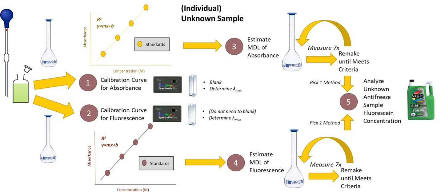
Visual Abstract

Background

Some molecules take in energy as light (absorbance) and then emit a different wavelength of light energy (emission). Fluorescence is a particular kind of emission where the release of energy happens between the same spin state (for example, between S₁→S₀). When a molecule fluoresces, emission occurs at longer wavelengths (or lower energy) compared to the excitation wavelength, since some of the excitation energy lost is due to vibrational relaxation. We can study this molecule via absorbance OR fluorescence, but molecules that can fluorescence is more rare and thus desirable to make sure the results are specific to the molecule of interest.

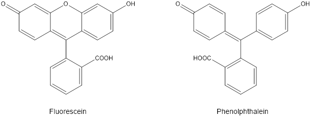
Fluorescein (Figure 1) is an organic compound used as a pigment (something that absorbs visible light and a fluorophore (a chemical that emits light) in a variety of products. Fluorescein is used to give yellow highlighters their bright color, it is frequently added to antifreeze for the radiator in your car so that leaks can be found, and it is used in medical research applications that use fluorescence as a way to tag biological molecules for detection.

Phenolphthalein, a classic colorimetric indicator for titrations is different from fluorescein only by one oxygen atom, which bridges two of the aromatic rings in the latter, as seen in Figure 1. This small structural difference changes the spectral behavior of fluorescein significantly: the result allows fluorescein to be used as an agent in fluorescence spectroscopy, whereas phenolphthalein does not fluoresce.

In this experiment you will compare and contrast spectra of fluorescein collected by absorption versus fluorescence spectrophotometry. Note from the structure shown in Figure 1 that fluorescein is also a weak acid. As a result, the fluorescence of this molecule exhibits a small pH dependence, within the range from pH 5 to 11. For this reason, as you make your samples from the stock solutions provided, be sure to use 0.1 M NaOH when making dilutions.

Quantitative Analysis & Quality Assurance

To perform a quantitative study, a set of standards of known concentration must first be made and measured. The resulting linear standard plot (called a calibration curve) can then be used to determine the concentration of the sample. In the case of absorbance measurements, absorbance and concentration are connected via the Beer-Lambert Law, also known as Beer’s Law. One process that limits the linear relationship between luminescence intensity and concentration is quenching, where neighboring molecules in a sample can absorb light from an excited molecule before the light can leave the cuvette, causing the analyte to absorbs its own fluorescence. Quenching is mainly an issue at higher concentrations, however, so intensity measurements are very linear at low concentrations.

In Beer’s Law, A is absorbance. ε is absorptivity of the molecule at a specific wavelength, which creates a wavelength-specific response for the absorbance. b is the pathlength of the instrument. c is the concentration of the molecule of interest. For fluorescence, a similar relationship exists, where intensity of the luminescence (I) is proportional to concentration (c) at a specific wavelength. The intensity (P₀) and wavelength (λ_excitation) of the incident radiation impact I and should remain constant when collecting standard and sample data.

Methods typically use the wavelength of maximum absorbance/intensity, λ_max, as the wavelength of analysis, since this produces the most sensitive assay. Standards measured at λ_max can be plotted and fit to a linear regression (y=mx+b) to make a calibration curve. Regardless of the method used, these points will only be linear in a specific range; the edges of this range are the upper and lower limits of linearity (see points 1 and 3 in Figure 2). In other words, outside of this range the signal stops increasing or decreasing proportionally to the concentration. Quantitation isn’t valid outside of the linear range (compare regions 4 and 5 in Figure 2), therefore, method development is necessary to ensure you’re working inside the linear range of the assay. Please note that you cannot report a concentration outside of your linear calibration curve. Instead, the sample should be concentrated or diluted so the signal falls within the correct range; when this is not possible, report “above/below the limit of linearity”.

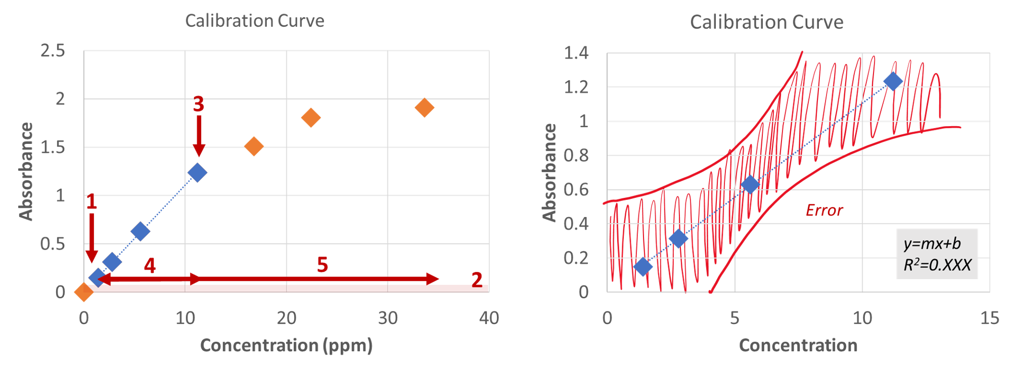
To have confidence in our method, we need to do quality assurance to make sure it is working properly. Beyond the linear range, it is a good practice to know the detection limit of the assay. The limit of detection is usually lower than the limit of linearity (see Point 1 in Figure 2 (left)). The detection limit (also known as the method detect limit (MDL) or limit of detection (LOD)), is the smallest quantity (i.e., concentration) of an analyte “significantly different” from the blank. Anything below the detection limit we report as either “0” or “below the detection limit”. The MDL is defined by that “wiggle” in the spectrum or the baseline noise (highlighted in Figure 4 and Figure 3-Region 2 (left)). That systematic error is captured in our calibration curve as the b-term, which is also why we do not want to force our calibration curve through zero. The MDL is calculated as

To have confidence in our method, we need to do quality assurance to make sure it is working properly. In addition to the linear range, it is a good practice to know the detection limit of the assay. The limit of detection (LOD) is the smallest quantity (i.e., concentration) of an analyte that can be confidently identified as “significantly different” from a blank. There are multiple types of limits of detection; we will focus on the method detection limit (MDL), which measures the limit of detection with regard to the entire method used. Other measures may only focus on a single part of the experiment: for example, an instrument detection limit (IDL) determines the quantity of sample an instrument can measure without regard for possible losses or variability in sample preparation. The MDL is usually lower than the limit of linearity (see point 1 in Figure 2), which means there is typically a range of concentrations where we can confidently report that analyte is present (i.e., the sample is not a blank), but we cannot determine the exact concentration.

MDL is calculated as

for 99% confidence for a one-tailed distribution and (n-1) degrees of freedom.¹ Carefully read the truncated procedure from the standard Environmental Protection Agency (EPA) procedure and use the method described there as guidance in determining the MDL for our method. Note that Equation 1 a Student’s t-value (t) based on the number of samples taken (n) and the standard deviation (s), which is a measure of the noise in our measurement.

Noise is the random variance in the signal when measured repeatedly. Where the signal of a blank is a systematic error (captured as the “b” term in a linear equation), we define noise as the random error present in all measurements. That random error will vary with the wavelength of interest and with the signal of the sample being measured; therefore, we must endeavor to measure this noise at the correct wavelength and at a concentration similar to the MDL itself. To do so, we’ll start with an estimate of the MDL and work recursively to find the true MDL.

First, we’ll need to find an estimate of the noise. We have two options.

1. Measure the blank (0.1 M NaOH in this case) 7 times (like the EPA method suggests) and determine the standard deviation of these measurements. This standard deviation will then be plugged into Equation 1 above.
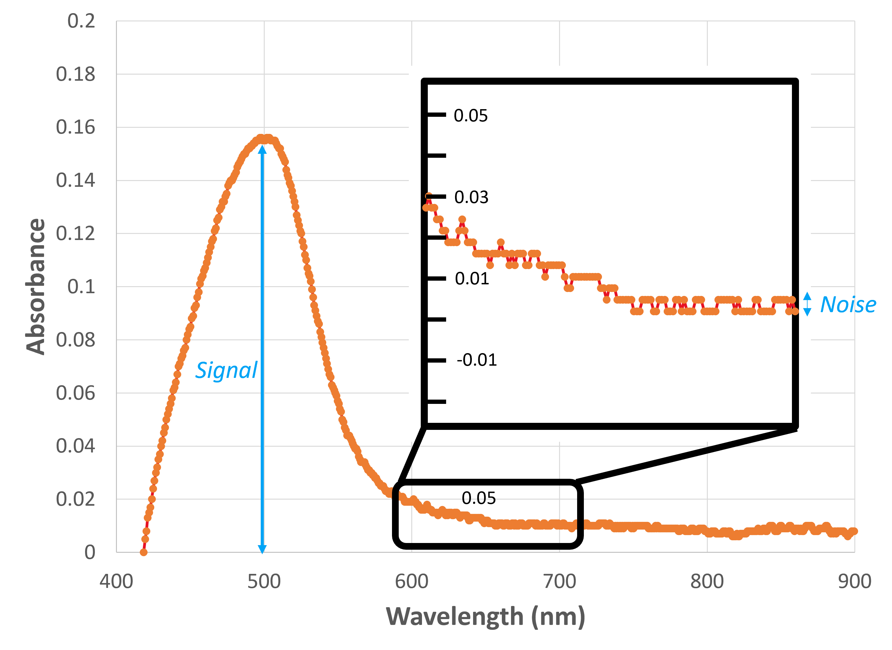
2. Look at a spectrum of a solution of known concentration and estimate the noise from the “wiggle” in a flat region (Figure 3 inset). Using our estimated noise and signal at the wavelength of interest, we can produce an estimated signal-to-noise (S/N) value of that sample. From there, assuming that the S/N scales linearly with concentration, we can estimate the concentration at the MDL by considering that, at the MDL, the S/N must be 2.5-5 (see EPA method).

Once we have this estimate, we can make a sample at this concentration estimate and then actually follow the EPA method by repeating this measurement. If all goes well, the MDL calculated will match the concentration used; this would confirm that the MDL is correct. If the values do not match, you must simply make a new solution at the new estimated concentration and repeat. How close you require the values to be depends upon the experiment; for our purposes, anything within a factor of 5 or so is probably fine.

[latex]\dfrac{S / N_1}{Concentration_1} = \dfrac{S / N_2}{Concentration_2}[/latex]

An example:
We make a blank sample at 0 uM, measure this 7 times, and determine an estimated MDL of 1.0 uM. 1.0 uM is very different from 0 uM, so we must continue.
We make a new sample at a concentration of 1.0 uM, measure this sample 7 times, and determine a new estimated MDL of 5.5 uM. 5.5 uM is very different from 1.0 uM, so we must continue.
We make a new sample at a concentration of 5.5 uM, measure this sample 7 times, and determine a new estimated MDL of 5.6 uM. 5.6 uM is close to 5.5 uM, so we can accept 5.6 uM as the MDL for our method!

Note that the amount of noise we get often varies with the strength of the signal. This is why we must use this trial-and-error method for determining the MDL.

Performing Serial Dilutions to Make Standards

Using serial dilutions to prepare a set of solutions (either for preparing samples or standards) is standard practice in the analytical lab. In using this method, you will perform successive dilutions of a stock standard (or sample).

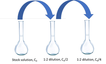
Consider Figure 4, for example, in preparing standards for this experiment using the stock solution provided. In this case we start with a solution that is 7.5 × 10^-5 M fluorescein. To achieve a set of standards using a serial dilution scheme using a 100 mL flask for the dilutions, one solution is to take 50 mL of the stock and dilute to 100 (a 50:100 or 1:2 dilution), resulting in 7.5 × 10^-5 M/2 = 3.7₅ × 10^-5 M fluorescein solution. Next, you can do the same thing with this second solution (i.e., take 50 mL and dilute to 100 mL, again a 1:2 dilution) resulting in a (3.7₅ × 10^-5 M) / 2 = 1.8₇ × 10^-5 M solution.

As you work to design your experiment for this lab, keep in mind the volumes of volumetric pipets available to you, which include 50, 25, 10, 5, 2, and 1 mL volumes. Other pieces of glassware can be used to perform the volume transfer of the previous solution, including a 1 mL Mohr pipet for small volumes, your Eppendorf pipets (potentially not as accurate as good old glassware!), or a buret.

In particular, this technique can be very important when trying to analyze a real-world sample, like antifreeze. You will not know what concentration/dilution is needed for analysis, and preparing a few serial dilutions to test is a good strategy!

More about the Instrument Used

Figure 5 illustrates the major internal components of the SpectroVis+ Vernier instrument, which can be used for both fluorescence and absorption spectroscopy applications.

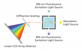
Notice that the excitation sources for fluorescence spectroscopy are offset 90° from the detector. This orientation minimizes the detection of scattered incident radiation, which is deflected by particles, the cuvette surface, and large molecules in solution. Notice that the instrument has 2 different light sources; in our case, the 500 nm excites fluorescein better than the 405 nm excitation source.

Lab Concept Video

Write your observations or notes from the video in your lab notebook.

Pre-lab Work

Lab Skills

Review these lab skills videos prior to lab.

Extra Resources:

• EPA Method Detection Limit Determination Procedure
• Using the LabQuest to Collect Spectrophotometry Data
• Making Scientific Plots

Prelaboratory Exercises

1. The stockroom will provide a stock solution of 7.5 × 10^-5 M fluorescein for preparing standard solutions. You will need to create a set of standards to calibrate the instrument in preparation for an absorption and fluorescence study of fluorescein. Use the table below to plan to make all the following solutions to be analyzed by both methods. Note that every solution will be made to 100 mL. Make sure you consider what pieces of glassware you have in the lab! Note that these concentrations are just estimates; If you make a dilution and a slightly different concentration, note that in the table below.
   

   Solution	Approximate Concentration	Dilution Plan	Actual Concentration
   1	75 uM
   2	37.5 uM
   3	18 uM
   4	7.5 nM
   5	3.75 uM
   6	1.5 uM
   7	0.75 uM
   8	0.075 uM
   9	0 uM

2. Consider the following intensity spectrum of fluorescein and phenolphthalein:
   
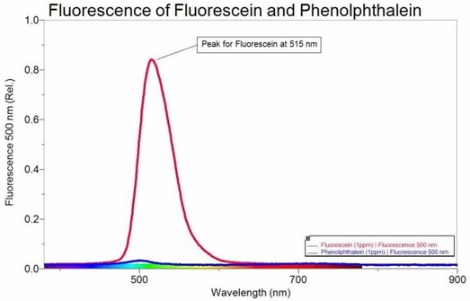
   Assuming a linear relationship is preserved between signal intensity and concentration, estimate in molarity units a detection limit for fluorescein (MW = 332.31) at 515 nm, using fluorescence spectroscopy. Remember your estimate should fall within a signal to noise range of 2.5 – 5.
3. What is the difference between the units of absorbance and relative intensity?

Before You Take The Quiz on Canvas

• Review the EPA Procedure for Method Detection Limit handout and understand how to determine a suitable, estimated detection limit.
• Have confidence in how to perform serial dilutions, and understand the process for performing this important technique.
• Understand how to calculate the concentration of an unknown sample given the fluorescence intensity of an unknown sample and a calibration curve of luminescing standards.
• Know the difference between absorption and fluorescence, and how these differences impact the instrumentation used for quantitative study.

Experimental

Part 1: Make the solutions as planned in Prelaboratory Question 1

1. As stated above. If you make any modifications, make sure you note that in your lab notebook. Make sure you dilute with 0.1 M NaOH (non-standardized is fine).

Part 2: Determine the method detection limit of fluorescein using fluorescence versus absorption spectroscopy

Determining the MDL for absorption spectroscopy

1. Using the 75 uM solution, determine the max wavelength for absorbance. Blank the instrument with the 0.1 M NaOH solution.
2. Once you have determined the wavelength of interest, measure all 9 solutions you prepared. Collect and save full wavelength spectra of your solutions.
3. Get an initial MDL via either method described in the background. Make a solution at that estimated concentration, and determine the MDL using the EPA procedure.

Determining the MDL for fluorescence spectroscopy

1. Using the 7.5 uM solution, determine the max wavelength for fluorescence using the 500 nm excitation source. Do NOT blank the instrument when the SpectroVis Plus is in fluorescence mode.
2. Once you have determined the wavelength of interest, measure all 9 solutions you prepared. Collect and save full wavelength spectra of your solutions.
3. Get an initial MDL via either method described in the background. Make a solution at that estimated concentration, and determine the MDL using the EPA procedure.

Part 3: Determine the concentration of fluorescein in commercial antifreeze

Obtain fluorescence intensity and/or absorbance measurements of a sample of commercial antifreeze.

1. To prepare your sample, begin by diluting 25 mL of sample to 100 mL using 0.1 M NaOH. Visually compare the resulting sample to your standards as a first guess as to whether you need to make more dilutions or not. Perform dilutions as needed until your sample concentration falls within the range of standards you prepared. Report the concentration of fluorescein in the ORIGINAL SAMPLE.

Post-Lab Work Up

Results/Calculations

Fill out the answer sheet for this experiment completely and answer the following post-lab questions.

1. Determine the wavelength maxima for each method (absorbance vs. fluorescence). Provide an example spectrum of each method to support your choice. Extract the absorbance and intensity at the max wavelength for each spectra.
2. Determine the linear range for both methods from the dynamic range. Make sure to include a copy of the final calibration curve (which should only include the linear range) in your submission. Suggest improvements to the procedure to optimize the calibration curves presented.
3. Report the MDL for each method, and comment upon which method is more sensitive in your reflective summary.
4. Using your method of choice (which is more sensitive? Which one has a better linear range? etc.), which should be justified in your reflective summary, quantify the amount of fluorescein in the antifreeze sample.

Challenge Questions

Challenge questions are designed to make you think deeper about the concepts you learned in this lab. There may be multiple answers to these questions! Any honest effort at answering the questions will be rewarded.

Beer’s law is useful in many additional contexts besides determining concentrations of analytes in solution. For example, Beer’s law governs light absorption in solid crystals, which in turn is relevant to many techniques that study the photophysical properties of materials. In lieu of molar concentration and absorptivity, absorbance of crystals depends instead on a material- and wavelength-dependent property called the absorption coefficient (α, in units of cm^-1) as well as the path length through the crystal (L), such that log(I₀/I) = αL.

Based on this information, answer the following questions to your best ability. Note that there are multiple ways of approaching these questions and that you are not expected to follow a particular method. As long as you show your reasoning, any honest attempt to answer each of these questions will be awarded full points.

1. Consider a monochromatic beam of violet light passing through a μm-sized, nm-thin red crystal of thickness L = 100 nm. Assume no light is reflected by the surface of the crystal, and let the absorption coefficient of the crystal for the wavelength of interest be α = 1.0 × 10⁵ cm^-1.
   
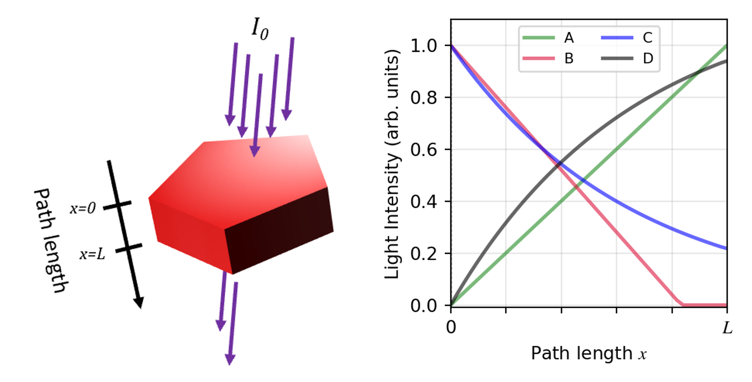
   1. Which of the plots, A-D, above best describes the evolution of the light intensity across the path length in the crystal? Based on the characteristics of the graph you chose (such as the slope or intercept), describe in detail how the intensity of light changes through the crystal.
   2. Draw a picture to show how you consider the light to interact with the crystal. Use the picture to provide a physical explanation for why the variation of light intensity with path length follows the plot you selected.
   3. Imagine for a moment the crystal in this problem fluoresces when excited by a 562.5 nm light source. Predict the color you might see with your eye and justify your answer with what you know about absorbance and fluorescence phenomenon.

Lab Report Submission Details

Submit your lab report on Canvas as 1 combined PDF file.  This submission should include:

1. The completed answer sheet.
2. Your lab notebook pages associated with this lab, which should include answers to the post-lab questions and challenge questions.

The grading rubric can be found on Canvas.

References:

1. Harris, D. C. & Lucy, C. A. Quantitative Chemical Analysis, 10^th ed.; W. H. Freeman: New York, NY, 2020