Beer’s Law Simulation
TOC/Help. Click here to expand/hide
Overview
Background
Pre-lab work
Experimental
Post-lab work
![]() For help before or during the lab, contact your instructors and TAs (detailed contact information are found on Canvas).
For help before or during the lab, contact your instructors and TAs (detailed contact information are found on Canvas).
Overview
In a guided-inquiry format, this lab uses a simple model to explore the phenomena of light interacting with sample contained in the cuvette and measured using a spectrophotometer. The result conveys a molecular understanding of the (a) fundamental process of absorption and (b) mathematical derivation of Beer’s Law.
Learning Objectives
- To describe the microscopic phenomenon of an absorption event in solution and corrolate the relationship of these events to absorbance spectroscopy, which lead to the Beer-Lambert Law.
- To explain chemistry and physics phenomena at a microscopic level by using a visual model.
To cite this lab manual: “Beer’s Law Simulation”. A Manual of Experiments for Analytical Chemistry. Department of Chemistry at UW- Madison, Summer 2024.
Visual Abstract
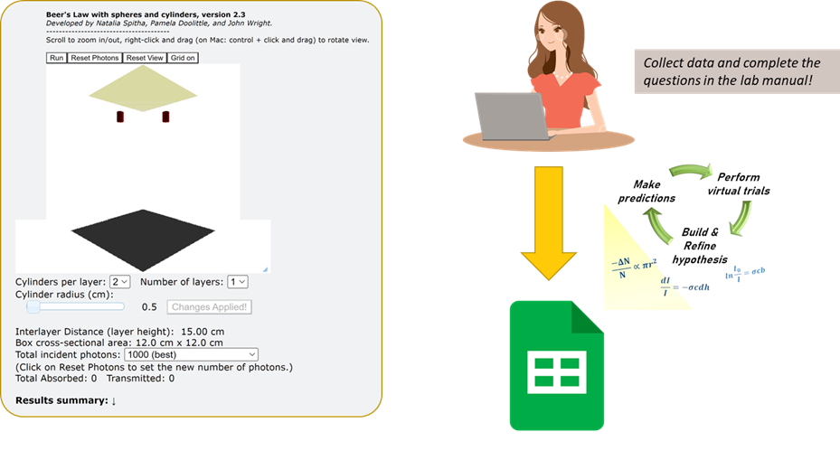

Background
Beer’s Law (also known as the Beer-Lambert Law) describes the relationship between the amount of light absorbed by a solution and its concentration. The absorbance (A) of a solution of concentration c in a cuvette with path length b is given by
| [latex]A = - \log \left(\dfrac{I}{I_0}\right) = \epsilon bc[/latex] | (1) |
where I0 is the intensity of light entering the solution, I is the intensity of the light exiting the solution, and ε is a constant called molar absorptivity, which is unique to each solute/solvent system. By now, you have probably held a cuvette and used it to measure the concentration of a solution using the principle of Beer’s law, but can you explain exactly what is going on in the cuvette at the molecular level? To help you visualize the process of absorption as well as provide a quantitative basis of what is occurring inside the cuvette, you will be interacting with a simulation that was hand-crafted here at UW-Madison.
The applet used in this lab simulates light going through a cuvette (i.e., a sample cell) by dropping small spheres (“photons”) through a box filled with cylinders (“solute particles”) arranged in a discrete number of layers. When a photon touches the surface of a cylinder, it gets stuck, emulating the absorption of light by a solute. The photons are arranged randomly along a single (x-y) plane and can move uniformly through the sample cell (z-direction). After “crossing” each layer, photon positions are always re-randomized along the x-y plane. The photons that are not captured by any cylinders make it through (are transmitted through) the cuvette and are detected by the screen on the bottom (the detector).
On screen, you will see a few buttons at the top, values you can edit on the bottom, and a running log about the data obtained from the simulation (very bottom). Every time you reload the simulation/web page, the box will be cleared.
The following controls will be useful:
- Run/Pause: starts or pauses the simulation
- Reset Photons: places the photons back at the “source,” allowing you to repeat the experiment. No need to click “Run” again if the simulation is already running.
- Reset View: resets the original view of the box (in case you zoomed in too much and got lost.)
- Update Cylinders: applies any changes you made to the number of layers or number/radius of cylinders and rearranges them in the box.
- Grid on/off: enables/disables a grid visualizing the box. Each square in the grid is 1 centimeter.
- You can also rotate the view of the cylinders by right-clicking and dragging anywhere inside the image.
It is recommended that, before starting the lab, you play around with the controls. See what values are given to you and try to resize the simulation. For good measures, see what happens when you don’t click Update Cylinders. If you understand the simulation controls, it will make it MUCH more efficient for you when collecting data from the simulation. You can do this as part of your pre-laboratory preparation!
Whenever we are collecting data in general, we have always wanted to collect replicates to understand how random error can impact a measurement. Thus, when assessing each set of conditions, make sure you perform at least 5 trials with 1000 photons each (7-8 trials is recommended). Also, as you know from learning the scientific process, there are logical steps for you to follow when trying to analyze a problem. Thus, we recommend the following already familiar steps in your lab notebook when answering each of the questions below:
- Create data tables to collect/log data (e.g., Figure 1) (We will supply some data already loaded into tables for you.)
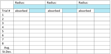
Figure 1. Example data collection table for experiments run with the simulation. - Collect data
- Perform calculations
- Critically evaluate the answer (e.g., Does the result make physical sense?)
- Phrase the answer in a sentence

Lab Concept Video
click here to hide the video (for printing purpose).
Data will be provided during the required "Lab Activities" Time if not provided in the video. Write down observations or notes from the video in your lab notebook.
Pre-lab Work
Lab Skills
Review these lab skills videos prior to lab.
click here to hide the video playlist (for printing purpose).
Key Takeaways
- Excel is a great tool to work up data!
Extra Resources:

Prelaboratory Exercises
- Briefly open the Beer’s Law simulation URL and take a look at the cylinder illustration and controls. This simulation serves as a model you can use to explain the Beer-Lambert relationship between light intensity (I/I0), concentration (c), molar absorptivity (ε), and path length (b). Identify and write down in your lab notebook how you think the quantities I, I0, c, ε, and b are represented in the simulation (that is, which properties of the spheres, cylinders, and box relate to each quantity).

Before You Take The Quiz on Canvas
- Watch all associated video content to introduce you to the simulation.
- Understand the basics of absorption spectroscopy, including the instrumental components, such as the light source, the cuvette, the sample, and the detector.
- Recognize Beer’s Law and be able to define what each variable means.
- Be able to convert between transmittance, percent transmittance, and absorbance.
Experimental
Open the Beer’s Law Simulation URL. Use the simulation to perform the virtual “experimental trials” listed below, remember to record your observations, calculations, and predictions in your notebook when prompted (usually, by underlined text). While the post-lab questions are at the end, you are welcome to answer and work through post-lab questions as you go along in the lab.
A starting data set is shared here for questions 1-4.
- For 1 layer with 2 cylinders, record the photons absorbed and transmitted for at least four different values of the cylinder radius with 1000 incident photons for each radius. Make sure you conduct enough trials. See an example data table in Figure 1.
- What do you predict the transmitted number of photons to be for 3 cylinders of radius 1.8 cm on one layer? Explain the reasoning for your prediction. Test your prediction by performing another set of trials.
In your lab notebook: Describe any relationship you observe between the radius of the cylinders and the number of absorbed or transmitted photons.If you find it difficult to identify a relationship with just your current sets of trials, or if your prediction was significantly off, feel free to select other radii or numbers of cylinders and run more trials until you feel comfortable you understand how the arrangement and size of cylinders affects the photons transmitted through a layer.
- For the same number and radius of cylinders per layer (3 cylinders, 1.8 cm), what do you predict the number of transmitted photons to be when you add a second layer for the photons to pass through? How about when a third layer is added? HINT: Remember that the photons captured by the first layer do not continue to the next layer! Test your hypothesis by performing another two sets of trials.
- Run a set of trials by setting the number of layers to 5, choosing a fixed cylinder radius >1.5 cm, and varying the number of cylinders per layer. Remember to conduct enough trials and to make a table!
- If you make a plot with the number of cylinders per layer on the x-axis, which dependent variable do you need to plot on the y-axis to obtain a linear, positive relationship according to Beer’s Law? Obtain 4 data points and test the linearity of your plot. HINT: the y-variable should NOT just be the number of photons absorbed!
Post-Lab Work Up

Results/Calculations
Answer the following post-lab questions as precisely as you can in your lab notebook.
- From the data collected in your Experimental step 1, determine a mathematical relationship that you can use to calculate the expected fraction of photons absorbed by one layer, given the number and radius of the cylinders as well as the total layer area.
- Explain why this relationship holds. HINT: What is the probability that a randomly positioned photon will get captured by a cylinder?
- How does your prediction from Experimental Step 2 compare with the result obtained? Using your result from question 1, explain why your prediction does or does not agree with the results.
- How do your predictions from Experimental Step 3 compare with the results obtained? Again, using the mathematical relationships you have discovered so far, explain why your prediction does or does not agree with the results.
- Using the mathematical relationship(s) you have determined, calculate how many transmitted photons one would expect to get in Experimental Step 3 (3 cylinders/layer, 1.8 cm) if (i) a fourth or (ii) a fifth layer was added (you don’t need to test this with the simulation). Sketch a plot of the expected number of transmitted photons against the number of layers. How would you describe the shape of that plot?
- Actual solutions have a continuous (rather than discrete) arrangement of molecules across their length. Let’s now put things in mathematical terms, to see how your above discoveries about cylinders neatly arranged in discrete layers can apply to a continuous situation. Consider the following variables:
- N = number of cylinders per cm3 (not per layer!)
- σ (sigma) = cross-sectional area of each cylinder in cm2
- A = cross-sectional area of each layer
- h = height of one layer
- b = total height of box
- I = number of photons transmitted
- I0 = total number of photons
Using the above variables:
- Express the volume of each layer.
- Express the number of cylinders per layer.
- Express the total cross-sectional area occupied by all cylinders in one layer.
- Based on your observations in Experimental steps 1-3 and Post-lab Question 6, what is the fractional change in number of transmitted photons (ΔΙ/Ι) passing through a single layer of thickness h? (HINT: It will be negative since photons are ‘lost’ via absorption.)
- Now consider your answer to Post-lab Question 7 for an infinitesimally small change in number of photons dI when passing a very thin layer of thickness dh. To find the number of photons transmitted through the entire sample (thickness b, initial number of photons I0), integrate both sides of that expression with respect to dI and dh. (HINT: This integration should give you Beer’s law!)
Math Help #1: [latex]\displaystyle {\int_{x = a}^{b} k \; dx = k ( b - a )}[/latex] Math Help #2: [latex]\displaystyle {\int_{x = a}^{b} \dfrac{1}{x} dx = \ln (b) - \ln (a)}[/latex] Math Help #3: [latex]\log_a (x) = \dfrac {\log_b (x)}{\log_b (a)}[/latex] Thus, Math Help #4: [latex]\log_{10} (x) = \dfrac{\ln (x)}{\ln (10)}[/latex] - From Experimental step 5, comment on the linearity of your collected data.
- How would your plot in Experimental step 5 change if the cylinder radius was increased? What property would this change be analogous to in a solution following Beer’s law?

Challenge Questions
Challenge questions are designed to make you think deeper about the concepts you learned in this lab. There may be multiple answers to these questions! Any honest effort at answering the questions will be rewarded.
- Do you have any additional improvements to propose for the simulation?
 Lab Report Submission Details
Submit your lab report on Canvas as 1 combined PDF file. This submission should include:
- The completed answer sheet.
- Your lab notebook pages associated with this lab, which should include answers to the post-lab questions and challenge questions.
The grading rubric can be found on Canvas.
References:
- Harris, D. C. & Lucy, C. A. Quantitative Chemical Analysis, 10th ed.; W. H. Freeman: New York, NY, 2020, page 62.
Please use this form to report any inconsistencies, errors, or other things you would like to change about this page. We appreciate your comments. 🙂 (Note that we cannot answer questions via the google form. If you have a question, please ask your instructor or TA.)
