
Part III. Spatial interactions on a grid
III-2. Robustness and fragility
1. Goal
Our goal in this chapter is to extend the model we have created in the previous chapter by adding three features that will prove very useful:
- Noise, i.e. the possibility that revising agents select a strategy at random with a small probability.
- Self-matching, i.e. the possibility to choose whether agents are matched with themselves to play the game or not.
- Asynchronous strategy updating, i.e. the possibility that agents revise their strategies sequentially –rather than simultaneously– within the same tick.[1]
These three features will allow us to assess the robustness of our previous computational results.
2. Motivation. Robustness of cooperation in spatial settings
In the previous chapter, we saw that spatial structure can induce significant levels of cooperation in the Prisoner’s Dilemma, at least for some parameter settings. In particular, we saw that with CD-payoff = DD-payoff = 0, CC-payoff = 1, DC-payoff = 1.85, the overall fraction of C-players fluctuates around 0.318 for most initial conditions (Nowak and May, 1992). Here we wonder how robust this result is to changes in some of the model assumptions. In particular, we would like to study what happens…
- if we add a bit of noise,
- if agents do not play the game with themselves,
- if strategy updating is asynchronous, rather than synchronous, or
- if we use DD-payoff = 0.1 (rather than DD-payoff = 0), making the game a true Prisoner’s Dilemma.
3. Description of the model
The model we are going to develop here is a generalization of the model implemented in the previous chapter. In particular, we are going to add the following three parameters:
- noise. With probability noise, the revising agent will adopt a random strategy; and with probability (1 – noise), the revising agent will choose her strategy following the imitate the best neighbor rule. Thus, if noise = 0, we recover the model implemented in the previous chapter.
- self-matching?. If self-matching? is true, agents play the game with themselves, just like before. On the other hand, if self-matching? is false, agents do not play the game with themselves.
- synchronous-updating?. If synchronous-updating? is true, agents update their strategies simultaneously, just like before. On the other hand, if synchronous-updating? is false, agents play and update their strategies sequentially, i.e. one after another. In this latter case, all agents revise their strategies in every tick in a random order.
Everything else stays as described in the previous chapter.
 4. Interface design
We depart from the model we developed in the previous chapter (so if you want to preserve it, now is a good time to duplicate it).
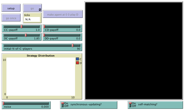
In the new interface (see figure 1 above), we just have to add one slider for the new parameter noise, and two switches: one for parameter synchronous-updating? and another one for parameter self-matching?. We have added these elements at the bottom of the interface, but feel free to place them wherever you like.
5. Code
5.1. Skeleton of the code
5.2. Extension I. Adding noise to the decision rule
Recall that the implementation of the decision rule is conducted in procedure to update-strategy-after-revision. At present, the code of this procedure looks as follows:
to update-strategy-after-revision
  set C-player?-after-revision
     [C-player?] of one-of my-nbrs-and-me with-max [payoff]
end
To implement the choice of a random strategy with probability noise by revising agents, we can use NetLogo primitive ifelse-value as follows:[2]
to update-strategy-after-revision
  set C-player?-after-revision ifelse-value (random-float 1 < noise)
    [ one-of [true false] ] ;; this is run with probability noise
    [ [C-player?] of one-of (my-nbrs-and-me with-max [payoff]) ]
end
The noise extension is now ready, so you may want to explore the impact of noise in this model.
5.3. Extension II. Playing the game with yourself or not
Whether it is natural to include self-interactions in the theory depends on the biological assumptions underlying the model. In general, if each cell is viewed as being occupied by a single individual adopting a given strategy then it is natural to exclude self-interaction. However, if each cell is viewed as being occupied by a population, all of whose members are adopting a given strategy, then it may be more natural to include self-interaction. Killingback and Doebeli (1996, p. 1136)
In our model, agents will play the game with themselves or not depending on the value of the new parameter self-matching?. To implement this extension elegantly, we find it convenient to define a new patch variable named my-coplayers, which will store the agentset with which the patch will play. Thus, if self-matching? is true, my-coplayers will include the patch’s neighbors plus the patch itself, while if self-matching? is false, my-coplayers will include only the patch’s neighbors.
It will also be convenient to define another patch variable named n-of-my-coplayers, which will store the cardinality of my-coplayers for each patch. This is just for the same (efficiency) reasons we defined n-of-my-nbrs-and-me in the previous model. Now that we have variables my-coplayers and n-of-my-coplayers, patch variable n-of-my-nbrs-and-me will no longer be needed. Thus, the definition of patch-own variables in the Code tab will look as follows:
patches-own [
  C-player?
  C-player?-after-revision
  payoff
  my-nbrs-and-me
  my-coplayers           ;; <== new variable
  n-of-my-coplayers      ;; <== new variable
  ;; n-of-my-nbrs-and-me    <== not needed anymore
]
Now we have to set the value of the two new patch-own variables. Since these values will not change during the course of the simulation and they pertain to the individual players, the natural place to set them is in procedure to setup-players.
to setup-players
  ask patches [
    set payoff 0
    set C-player? false
    set C-player?-after-revision false
    set my-nbrs-and-me (patch-set neighbors self)

    ;; set n-of-my-nbrs-and-me (count my-nbrs-and-me)  <== not needed anymore
    ;; the following two lines are new
    set my-coplayers ifelse-value self-matching? [my-nbrs-and-me] [neighbors]
    set n-of-my-coplayers (count my-coplayers)
  ]
  ask n-of (round (initial-%-of-C-players * count patches / 100)) patches [
    set C-player? true
    set C-player?-after-revision true
  ]
end
Finally, we have to modify procedure to play so patches play with agentset my-coplayers, rather than with agentset my-nbrs-and-me.
to play
  let n-of-C-players count my-coplayers with [C-player?]
  set payoff
      n-of-C-players * (ifelse-value C-player? [CC-payoff] [DC-payoff]) +
      (n-of-my-coplayers - n-of-C-players) *
          ifelse-value C-player? [CD-payoff] [DD-payoff]
end
Note also that we have to replace the variable n-of-my-nbrs-and-me with n-of-my-coplayers when computing the payoff. You can now explore the consequences of not forcing agents to play the game with themselves!
5.4. Extension III. Asynchronous strategy updating
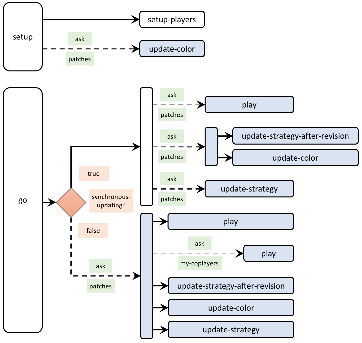
To implement asynchronous updating we will have to modify procedure to go. If synchronous-updating? is true, updating takes place just like before, so we can wrap the code we had in to go within an ifelse statement whose condition is the boolean variable synchronous-updating? , i.e.:
to go
  ifelse synchronous-updating?
    [
      ask patches [ play ]
      ask patches [
        update-strategy-after-revision
          ;; here we are not updating the agent's strategy yet
        update-color
      ]
      ask patches [ update-strategy ]
        ;; now we update every agent's strategy at the same time
    ]
    [
      ;; this is where we have to place the code
      ;; for asynchronous strategy updating
    ]
  tick
end
The implementation of sequential updating requires that every patch (in a random order) goes through the whole cycle of playing and updating its strategy without being interrupted. Note that, at the time of revising the strategy, agents will compare their payoff with their coplayers’ payoffs, so before calling procedure update-strategy-after-revision we have to make sure that all these payoffs have been properly computed, i.e. we must ask the revising agent and her coplayers to play the game. So basically, each patch, in sequential order, must:
- play the game,
- ask its coplayers to play the game (so their payoffs are updated),
- run update-strategy-after-revision to compute its next strategy (C-player?-after-revision),
- update its color (now that we have access both to the current strategy C-player? and to the next strategy C-player?-after-revision)
- update its strategy, i.e. set the value of C-player? to C-player?-after-revision. This is done in procedure update-strategy.
Taking all this into account, the code in the procedure to go looks as follows:
to go
  ifelse synchronous-updating?
    [
      ask patches [ play ]
      ask patches [
        update-strategy-after-revision
          ;; here we are not updating the agent's strategy yet
        update-color
      ]
      ask patches [ update-strategy ]
        ;; now we update every agent's strategy at the same time
    ]
    [
      ask patches [
        play
        ask my-coplayers [ play ]
           ;; since your coplayers' strategies or
           ;; your coplayers' coplayers' strategies
           ;; could have changed since the last time
           ;; your coplayers played
        update-strategy-after-revision
        update-color
        update-strategy
      ]
    ]
  tick
end
5.5. Complete code in the Code tab
The Code tab is ready! Congratulations! You have implemented three important generalizations of the model in very little time.
patches-own [
  C-player?
  C-player?-after-revision
  payoff
  my-nbrs-and-me
  my-coplayers
  n-of-my-coplayers
]

to setup
  clear-all
  setup-players
  ask patches [update-color]
  reset-ticks
end

to setup-players
  ask patches [
    set payoff 0
    set C-player? false
    set C-player?-after-revision false
    set my-nbrs-and-me (patch-set neighbors self)
    set my-coplayers ifelse-value self-matching? [my-nbrs-and-me] [neighbors]
    set n-of-my-coplayers (count my-coplayers)
  ]
  ask n-of (round (initial-%-of-C-players * count patches / 100)) patches [
    set C-player? true
    set C-player?-after-revision true
  ]
end

to go
  ifelse synchronous-updating?
    [
      ask patches [ play ]
      ask patches [
        update-strategy-after-revision
          ;; here we are not updating the agent's strategy yet
        update-color
      ]
      ask patches [ update-strategy ]
        ;; now we update every agent's strategy at the same time
    ]
    [
      ask patches [
        play
        ask my-coplayers [ play ]
           ;; since your coplayers' strategies or
           ;; your coplayers' coplayers' strategies
           ;; could have changed since the last time
           ;; your coplayers played
        update-strategy-after-revision
        update-color
        update-strategy
      ]
    ]
  tick
end

to play
  let n-of-cooperators count my-coplayers with [C-player?]
  set payoff
      n-of-cooperators * (ifelse-value C-player? [CC-payoff] [DC-payoff]) +
      (n-of-my-coplayers - n-of-cooperators) *
           ifelse-value C-player? [CD-payoff] [DD-payoff]
end

to update-strategy-after-revision
  set C-player?-after-revision ifelse-value (random-float 1 < noise)
    [ one-of [true false] ]
    [ [C-player?] of one-of (my-nbrs-and-me with-max [payoff]) ]
end

to update-strategy
  set C-player? C-player?-after-revision
end

to update-color
  set pcolor
    ifelse-value C-player?-after-revision
     [ifelse-value C-player? [blue] [lime]]
     [ifelse-value C-player? [yellow] [red]]
end
6. Sample runs
Now that we have implemented the extended model, we can use it to answer the questions posed in the motivation above. Let us see how the simulation we ran in the previous chapter (with CD-payoff = DD-payoff = 0, CC-payoff = 1, DC-payoff = 1.85, and initial-%-of-C-players = 90 in a 81×81 grid) is affected by each of the changes outlined in the motivation, one by one. We will refer to this parameterization as the baseline setting.
What happens if we add a bit of noise?
If you run the model with noise, you will see that the level of cooperation diminishes drastically. Using BehaviorSpace, we have estimated that the percentage of cooperators in the regime where cooperators and defectors coexist drops from ~32% in the model without noise to ~15% if noise = 0.04. If noise = 0.05, the long-run fraction of cooperation is just ~3%, so nearly all cooperation is coming from the random strategy updates (which accounts for 2.5% of the cooperation).[3] The influence of noise in the baseline setting was pointed out by Mukherji et al. (1996).
What happens if agents do not play the game with themselves?
The impact of self-matching? is also clear. When agents do not play the game with themselves, no cooperation can emerge in the baseline setting. If the initial fraction of cooperators is high, some small clusters of initial cooperators may survive, but these clusters disappear if we add a tiny bit of noise. As an illustration, the video below shows a simulation with self-matching? = false, initial-%-of-C-players = 99 and noise = 0.01.
Therefore, it turns out that playing with oneself is a necessary condition to obtain some cooperation in the baseline setting.
What happens if strategy updating is asynchronous, rather than synchronous?
The impact of synchronous-updating? on cooperation is also clear. If agents update their strategies sequentially, rather than simultaneously, no cooperation whatsoever can be sustained in the baseline setting. This observation was pointed out by Huberman and Glance (1993). As a matter of fact, to eliminate cooperation in this setting, it is sufficient that only a small fraction of the population (~15%) do not synchronize (Mukherji et al., 1996).[4]
What happens if we use DD-payoff = 0.1?
Increasing the value of DD-payoff to 0.1 (so the game becomes a real Prisoner’s Dilemma) also eliminates the emergence of cooperation. If the initial fraction of cooperators is high, some small clusters of initial cooperators may survive, but these clusters disappear if we add some noise.[5] As an illustration, the video below shows a simulation with DD-payoff = 0.1, initial-%-of-C-players = 99 and noise = 0.01.
Discussion
In this chapter we have discovered that the emergence of cooperation observed in the sample run of the previous chapter is not robust at all. Any of the four modifications we have explored is sufficient to destroy cooperation altogether. Having said that, the emergence of cooperation in the spatially embedded Prisoner’s Dilemma is much more robust for lower values of DC-payoff (see Nowak et al. (1994a, 1994b, 1996)). As an example, consider a simulation with DC-payoff = 1.3, where we include the four modifications we have investigated, i.e. noise = 0.05, self-matching? = false, synchronous-updating? = false, and DD-payoff = 0.1. The other parameter values are the same as in our baseline simulation, i.e. CD-payoff = 0, CC-payoff = 1, and the grid is 81×81. Cooperation in this setting can indeed emerge and be sustained. The video below shows an illustrative run with initial conditions initial-%-of-C-players = 25. The long-run proportion of cooperators in this setting is greater than 50%.
In chapter III-4 we will see that there is another assumption in this model that has a very important (positive) influence in the emergence of cooperation: the use of the imitate the best neighbor rule. But for now, let us take a step back and think about what we have learned in this chapter in general terms, i.e. beyond the specifics of this particular model.
In this chapter we have learned that assumptions that may seem irrelevant at first sight can actually play a crucial role in the dynamics of our models. Furthermore, there are often complex interactions between the effects of different assumptions. We have also learned that small changes in one parameter can lead to big changes in the dynamics of our models (see exercise 1 below for a striking example). Unfortunately, this sensitivity to seemingly small details is not the exception but the rule in agent-based models. For this reason, it is of utmost importance to always check the robustness of our computational results, to explore the parameter space adequately, and to keep our conclusions within the scope of what we have actually investigated, not beyond.
7. Exercises
You can use the following link to download the complete NetLogo model: 2×2-imitate-best-nbr-extended.nlogo.

Exercise 1. Roca et al. (2009a, fig. 10; 2009b, fig. 2) report a counterintuitive singularity that we can replicate with our model. To do so, modify the baseline setting (CD-payoff = DD-payoff = 0, CC-payoff = 1) by choosing self-matching? = false, make the world 100×100 with periodic (or ‘wrap-around’) boundaries, and set initial conditions initial-%-of-C-players = 50. Now compare the long-run fraction of cooperators for values of DC-payoff equal to 1.3999, 1.4 and 1.4001. What do you observe?
To understand this curious phenomenon, you may also want to run simulations with initial conditions initial-%-of-C-players = 100 and make use of our button labeled .
P.S. One may wonder whether this singularity could be an artifact due to floating-point errors, since (1.4 + 1.4 + 1.4 + 1.4 + 1.4) ≠ 7 in the IEEE754 floating-point standard (which is the standard used in most programming languages, and in NetLogo in particular).[6] You can check that the singularity is not due to floating-point errors choosing an equivalent parameterization that is not prone to floating-point errors. Can you come up with an equivalent parameterization that uses only integers when computing payoffs?
Exercise 2. Consider the simulation run from the previous chapter which produced the beautiful kaleidoscopic patterns. How does each of the four modifications outlined in the motivation affect its dynamics?
Exercise 3. How can we parameterize our model to replicate the results shown in figure 2 of Killingback and Doebeli (1996, p. 1138)?
![]() Exercise 4. What changes should we make in the code to be able to replicate figure 3 of Killingback and Doebeli (1996, p. 1139)? Note that in the model used to produce that figure, individual patches do not update their strategy with 5% probability.
Exercise 4. What changes should we make in the code to be able to replicate figure 3 of Killingback and Doebeli (1996, p. 1139)? Note that in the model used to produce that figure, individual patches do not update their strategy with 5% probability.
![]() Exercise 5. In section “Sample runs”, when we added some noise to the baseline setting, we stated that the percentage of cooperators in the regime where cooperators and defectors coexist is about ~15% if noise = 0.04. Try to corroborate this estimation using BehaviorSpace.
Exercise 5. In section “Sample runs”, when we added some noise to the baseline setting, we stated that the percentage of cooperators in the regime where cooperators and defectors coexist is about ~15% if noise = 0.04. Try to corroborate this estimation using BehaviorSpace.
![]() Exercise 6. In our model, changing the value of noise has an immediate effect on the dynamics of the model at runtime. The same occurs with synchronous-updating?, but not with self-matching?. How can you make the model respond immediately to changes in self-matching? ? Try to do it in a way that does not affect the execution speed.
Exercise 6. In our model, changing the value of noise has an immediate effect on the dynamics of the model at runtime. The same occurs with synchronous-updating?, but not with self-matching?. How can you make the model respond immediately to changes in self-matching? ? Try to do it in a way that does not affect the execution speed.
- There are different ways one can implement asynchronicity. Here we implement what Cornforth et al. (2005) call "Random Asynchronous Order". Under this scheme, at each tick all agents revise their strategy in a random order. ↵
- We could also implement the noise extension using the NetLogo primitive ifelse, but the use of ifelse-value makes it clear that the only thing we are doing in this procedure is to set the value of the patch variable C-player?-after-revision. ↵
- The model with low noise seems to have two regimes, one where most agents are defecting and another one where cooperators and defectors coexist. Simulations that start with a low percentage of initial cooperators tend to move first to the mostly-defection regime, while simulations that start with higher proportions of initial cooperators tend to move to the coexistence regime. Note, however, that transitions from one regime to the other are always possible with noise, and therefore they will occur if we wait for long enough. Having said that, the time we would have to wait to actually see these transitions may be extremely long in some settings. Note also that the model with noise can be seen as an irreducible and aperiodic Markov chain (see sufficient conditions for irreducibility and aperiodicity). This means that the long-run dynamics of this model are independent of initial conditions. ↵
- Newth and Cornforth (2009) analyze various other updating schemes in this model. ↵
- If DD-payoff
 0.58, no clusters of initial cooperators can survive, even in the absence of noise. ↵
 - Note that in our implementation of procedure to play we do not add individual payoffs but we multiply them, so we would not compute (1.4 + 1.4 + 1.4 + 1.4 + 1.4) but instead 5*1.4, which is indeed exactly equal to 7 in IEEE754 floating-point arithmetic. For more on the potential impact of floating-point errors on agent-based models, see Polhill et al. (2006) and Izquierdo and Polhill (2006). ↵
