
Part IV. Games on networks
IV-5. Analysis of these models
1. Introduction
In Part II, we learned to implement and analyze models in well-mixed populations. These are models where every agent has the same probability of interacting with every other agent. In such models, the state of the system can be defined by the distribution of strategies in the population; in other words, the strategy distribution contains all the information we need to (probabilistically) predict the evolution of the system as accurately as it is possible. Because of this, we saw that there are various mathematical techniques that we can use to analyze and characterize the dynamics of these models impressively well (see chapter II-5). For well mixed populations, the usefulness of mathematical analysis cannot be overstated.
In Part III, we learned to implement and analyze models on spatial grids. In these models, the strategy distribution is not enough to predict the evolution of the system anymore because each agent has its own set of neighbors (see chapter III-5). Nonetheless, in grid models there is still some symmetry in the sense that all agents have the same number of neighbors (except, maybe, at the boundaries). Because of this, for some of these models, we could still derive some analytical approximations such as the pair approximation for regular networks. These approximations can be useful because they are sometimes able to predict overall trends, but in general there is no guarantee that they will work well. For this reason, the relative usefulness of the computer simulation approach as a tool for exploration and analysis (vs the mathematical approach) is significantly greater in spatial models than in well-mixed populations.
Finally, here in Part IV, we have learned to implement models where agents are embedded on arbitrary networks. In these models, each agent has its own set of neighbors and, in general, there is no symmetry whatsoever, so the state of the system must be defined at the individual level. Because of this, the mathematical approach loses much of its usefulness and we are bound to resort to computer simulation as the main tool for exploration and analysis.
The challenge is high, because heterogeneity in both agent types and connectivity structure breaks down the symmetry of agents, and thus requires a dramatic change of perspective in the description of the system from the aggregate level to the agent level. The resulting huge increase in the relevant system variables makes most standard analytical techniques, operating with differential equations, fixed points, etc., largely inapplicable. What remains is agent based modeling, meaning extensive numerical simulations and analytical techniques going beyond the traditional mean-field level. Szabó and Fáth (2007, p. 102)
In this chapter, we are going to illustrate the importance of four best practices that we should try to follow when using the computer simulation approach:
- Avoid errors
- Use informative metrics
- Report meaningful statistics
- Derive sound conclusions
Let us see each of these in turn!
2. Avoid errors
2.1. Introduction
Following Galán et al. (2009, par. 3.3), we consider that an error has occurred whenever there is a mismatch between what the model does and what we, developers, think the model does. Naturally, we should always try to avoid errors.
The most common errors are those that we inadvertently introduce in our code, i.e., situations where we are telling the computer to do something different from what we want it to do. We have seen several examples of this type of coding error in this book. For example, in our very first model (chapter II-1), we initially discussed a natural but faulty implementation of procedure to go, where some strategies could be imitated based on payoffs that had not been obtained with those strategies (see section “A naive implementation“). To fix this error we defined a new agents’ variable named strategy-after-revision.
In section 5.7 of that same chapter, we saw another error. At first, we did not properly initialize the agents’ variable strategy-after-revision, and that led to dynamics that were not the ones we intended to implement. You can find other examples of errors (and their fix) in chapter IV-1, where our code could ask players with no neighbors to select one of them, and in chapter IV-2, where our code could try to select 15 agents out of a set of only 5.
Galán et al. (2009) discuss several activities aimed at detecting and avoiding errors in agent-based models, including reimplementing the model in different programming languages and testing the model in extreme cases that are perfectly understood (Gilbert and Terna, 2000). Examples of extreme cases that are often easy to understand include setting the probability of revision equal to 0, setting all payoffs to 0, or setting the noise to 1.
Here we would like to discuss a subtle type of error that is often neglected, but which can have undesirable consequences that may be difficult to detect and understand, i.e., floating-point errors.
2.2. Floating-point errors
Like most programming languages, NetLogo represents numbers internally in base 2 (using 64-bit strings) and adheres to the IEEE standard for floating-point arithmetic (IEEE 754).[1] This means, in particular, that any number that is not exactly representable in base 2 with a finite bitstring cannot be exactly stored in NetLogo. Some examples of decimal numbers that cannot be represented exactly with a finite bitstring are 0.1, 0.2, 0.3, 0.4, 0.6, 0.7, 0.8, and 0.9. As a matter of fact, only 63 of the 999 999 numbers of the form 0.000001·i (i = 1, 2… 999 999) are exactly representable in IEEE 754 single or double precision. Thus, whenever we input one of these numbers in our model, we are inevitably introducing some rounding error. This error will generally be very small, but when dealing with discontinuous functions, small errors can have big consequences.
Example 1. As an example, consider the imitate if better decision rule, which dictates that an agent A will copy the strategy of an observed agent B if and only if the observed agent B has a greater payoff. Now imagine that agents obtain a payoff by playing three times, and agent A’s payoff is (0.3 + 0 + 0) while agent B’s payoff is (0.1 + 0.1 + 0.1). It turns out that the IEEE 754 floating-point result of the sum (0.1 + 0.1 + 0.1) is slightly greater than the floating-point result of the sum (0.3 + 0 + 0). You can check this by typing the following lines in the command center of NetLogo:[2]
show (0.1 + 0.1 + 0.1)
show (0.1 + 0.1 + 0.1) > (0.3 + 0 + 0)
Therefore, in this particular example, agent A would copy agent B’s strategy, but it should not copy it according to real arithmetic. Let us emphasize that this is not a problem specific to NetLogo. You would get the same result in any IEEE 754-compliant platform.
Example 2. To see floating-point errors in action in one of our models, you can run our last model with payoffs [[0 1.2] [-0.2 1]] and, after a few ticks, check the agents’ payoffs by typing the following line in the command center:
show sort remove-duplicates [payoff] of players
When we do this, we get numbers such as -0.20000000000000018, 0.19999999999999996, 0.3999999999999999, 1.5999999999999999, or 1.7999999999999998 (and also numbers very close to these, such as 1.6 and 1.8). By contrast, if you run the same model with the payoffs we used in the sample runs ([[0 1.1875] [-0.1875 1]]), you will not find any floating-point errors. This is the reason we chose these payoff values.
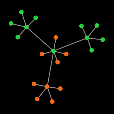
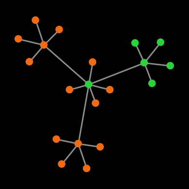
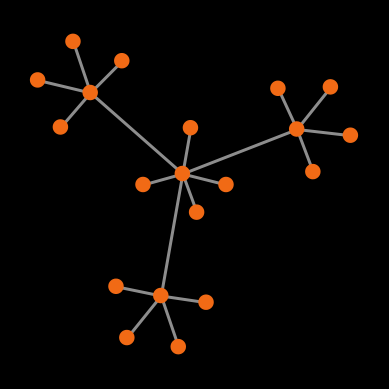
Example 3. Let us finish with a full-fledged example. Consider the Prisoner’s dilemma [[0 1.2] [-0.4 1]] played on the network shown in figure 1 below, using total (accumulated) payoffs. Green nodes are cooperators and red nodes are defectors.
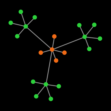
The payoffs for the different agents are:
| Type of agent | Payoff computation | Payoff value (exact arithmetic) |
Payoff value (floating-point arithmetic) |
|---|---|---|---|
| Cooperating hubs | 4 * 1 + 1 * (-0.4) | 3.6 | 3.6 [3] |
| Defecting hub | 4 * 0 + 3 * 1.2 | 3.6 | 3.5999999999999996 |
| Cooperating leaves | 1 * 1 | 1 | 1 |
| Defecting leaves | 1 * 0 | 0 | 0 |
Looking at the payoffs for the different agents above, we know that under decision rules imitate the best neighbor and imitate if better, the defecting hub will imitate one of the cooperating hubs (since 3.6 > 3.5999999999999996), and then the defecting leaves will follow suit. Thus, under these two decision rules, using IEEE 754 floating-point arithmetic, the population will always evolve to a state of full cooperation.
However, under real arithmetic, the end state of these simulations is very different. If agents use the imitate if better rule, the population will stay in the initial state forever; and if agents use the imitate the best neighbor rule, the simulation will end up in one of a set of four possible end states (allowing for symmetries). Table 1 below shows the probability of ending up in each of the possible different end states, assuming prob-revision = 1.
| End state | 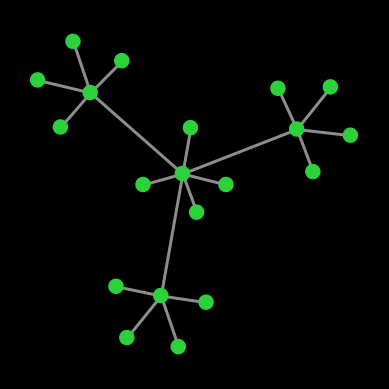 |
 |
 |
 |
| Number of cooperators | 20 | 11 | 6 | 0 |
| Probability | 9.68 % | 38.71 % | 38.71 % | 12.90 % |
Table 1. Possible end states and their probabilities for a population of agents playing the Prisoner’s dilemma with payoffs [[0 1.2] [-0.4 1]], using total (accumulated) payoffs and the imitate the best neighbor rule. Initial conditions are shown in figure 1 and prob-revision = 1. States that differ on a rotation of the network are lumped together
It is clear that the results obtained with floating-point arithmetic are completely different from those obtained with real arithmetic. A simple way to avoid floating-point errors in this particular example would be to multiply all payoffs by 10. This is a good practice in general: if we have the freedom to do so, we should try to parameterize models using numbers that are exactly representable in base 2. For instance, if we want to explore different values of a parameter that ranges from 0 to 1, we should do it in steps of 0.125, rather than in steps of 0.1.
Nonetheless, it is also important to note that not all models are equally susceptible to floating-point errors, by any means. Decision rules such as the imitative pairwise-difference rule, the Fermi-m rule or the Santos-Pacheco rule are continuous in the sense that small changes in payoffs will lead to small changes in agents’ behavior. Since floating-point errors in these models are often very small in magnitude, their impact on agents’ behavior will also be small. Therefore, continuous models are not usually severely affected by floating-point errors.
To learn more about the potential impact of floating-point errors on agent-based models, see Polhill et al. (2006) and Izquierdo and Polhill (2006).
3. Use informative metrics
3.1. Metrics
We obtain information from simulation models by using metrics. Metrics here are just measurements of some aspect of the dynamics, such as the proportion of players using a certain strategy:
count players with [strategy = 1] / count players
These metrics could refer to one particular tick or to several ticks. For instance, it is common to measure the average proportion of players using a certain strategy over a certain period of time, since averages tend to have lower variability than single observations at a particular tick. This can be easily done in NetLogo as follows:
globals [
  ...
  first-tick-of-report
  last-tick-of-report
  cumulative-x1
]

to setup
  ...
  setup-reporters
end

to go
  ...
  tick
  update-reporters
  ...
end

;;;;;;;;;;;;;;;;;;;;;;;;
;;;    Reporters     ;;;
;;;;;;;;;;;;;;;;;;;;;;;;

to setup-reporters
  set first-tick-of-report 10001
  set last-tick-of-report  11000
set cumulative-x1 0
end
to update-reporters
  if (ticks >= first-tick-of-report and ticks <= last-tick-of-report) [
    let x1 count players with [strategy = 1] / count players
    set cumulative-x1 (cumulative-x1 + x1)
  ]
end

to-report avg-x1
  report cumulative-x1 / (last-tick-of-report - first-tick-of-report + 1)
end
The code additions above ensure that, after tick last-tick-of-report, variable cumulative-x1 will contain the sum of all the values of x1 from first-tick-of-report up until last-tick-of-report, both inclusive. So, if called after tick last-tick-of-report, reporter avg-x1 will return the average proportion of players using strategy 1 in the interval [first-tick-of-report , last-tick-of-report]. We can then use reporter avg-x1 as a metric in BehaviorSpace.
3.2. Stability of metrics
Naturally, our metrics should measure something that is informative for our purposes. Here we comment on one aspect of metrics that is specially relevant in dynamic models: their stability. Most often, we wish to report a metric when its value has stabilized. There is nothing wrong in reporting the value of a metric when it is not yet stable, but the metric is usually more informative if we know that the reported value will not change much in future time-steps. How do we know if a metric has stabilized? One way is to compute the metric at a later tick in the same simulation and compare the two values. If the second value is systematically greater or smaller than the first value, then this is a strong indication that the metric has not yet stabilized. Let us see this with an example.
Consider the last model we have implemented (nxn-games-on-networks.nlogo), parameterized as follows:
["n-of-players-for-each-strategy" "[5000 5000]"]
["payoffs" "[[0 1.1]\n [0 1]]"]
["network-model" "preferential-attachment"]
["min-degree" 2]
["decision-rule" "imitative-pairwise-difference"]
["play-with" "all-nbrs-AVG-payoff"]
["prob-revision" 1]
["noise" 0]
This is a setting that corresponds to value b = 1.1 in figure 6 of Santos and Pacheco (2006) for the Barabási-Albert network. The value reported in that figure is the average proportion of cooperators over the period that goes from tick 10 001 to tick 11 000, and it is slightly greater than 20%.[4] To see whether this 1000-tick average is reasonably stable after 10 000 ticks, we can compute the same average starting at a later tick and compare the two averages for each simulation run. We can do this using the following code, which is not particularly elegant or efficient, but it will do the job:
globals [
  ...
  ;; for first metric
  first-tick-of-report
  last-tick-of-report
  cumulative-x1

  ;; for second metric
  first-tick-of-report-2
  last-tick-of-report-2
  cumulative-x1-2
]

to setup
  ...
  setup-reporters
end

to go
  ...
  tick
  update-reporters
  ...
end

;;;;;;;;;;;;;;;;;;;;;;;;
;;;    Reporters     ;;;
;;;;;;;;;;;;;;;;;;;;;;;;

to setup-reporters
  ;; for first metric
  set first-tick-of-report 10001
  set last-tick-of-report  11000
  set cumulative-x1 0

  ;; for second metric
  set first-tick-of-report-2 11001
  set last-tick-of-report-2  12000
  set cumulative-x1-2 0
end

to update-reporters
  let x1 count players with [strategy = 1] / count players

  ;; for first metric
  if (ticks >= first-tick-of-report and ticks <= last-tick-of-report) [
    set cumulative-x1 (cumulative-x1 + x1)
  ]

  ;; for second metric
  if (ticks >= first-tick-of-report-2 and ticks <= last-tick-of-report-2) [
    set cumulative-x1-2 (cumulative-x1-2 + x1)
  ]
end

;; for first metric
to-report avg-x1
  report cumulative-x1 / (last-tick-of-report - first-tick-of-report + 1)
end

;; for second metric
to-report avg-x1-2
report cumulative-x1-2 / (last-tick-of-report-2 - first-tick-of-report-2 + 1)
end
We have run 100 simulations and obtained that the second average (avg-x2) was greater than the first one (avg-x1) in 91 runs, which suggests that the value is still increasing by tick 10 000. If the metric was stable by tick 10 000, we would expect the second average to be greater in approximately 50 runs (or fewer, if ties are likely). If the metric was stable, we would observe the result we have obtained (91/100 runs), or an even more extreme result, with probability less than 10-17.[5] Thus, this computational experiment provides very strong evidence against the hypothesis that the metric is stable by tick 10 000.
Figure 2 below shows a representative run of this setting, with a vertical black line at tick 10 000. It is clear that the proportion of cooperators (in green) has not stabilized by tick 10 000. In this run, the average proportion of cooperators is 23.6% over the period [10 001 , 11 000], but significantly higher afterwards (e.g., 33.9% over the period [110 001 , 111 000]).
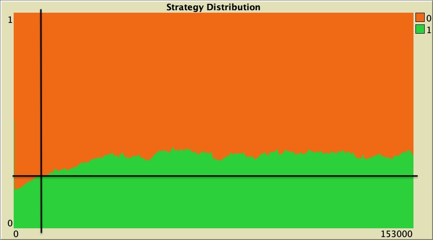
As a conclusion, we recommend to check the stability of reported metrics, as we have done here. It is a reasonably simple test that will make the metrics we report more informative.
4. Report meaningful statistics
When we run a stochastic model, we are usually interested in finding out not only how the model can behave, but also how it usually behaves. For this, we run many simulation runs and compute different statistics on the metrics obtained from each run. A statistic is any quantity computed from values in a sample. Here the sample consists of the values of a certain metric obtained from each of the simulation runs in the experiment. An example of a statistic is the average.
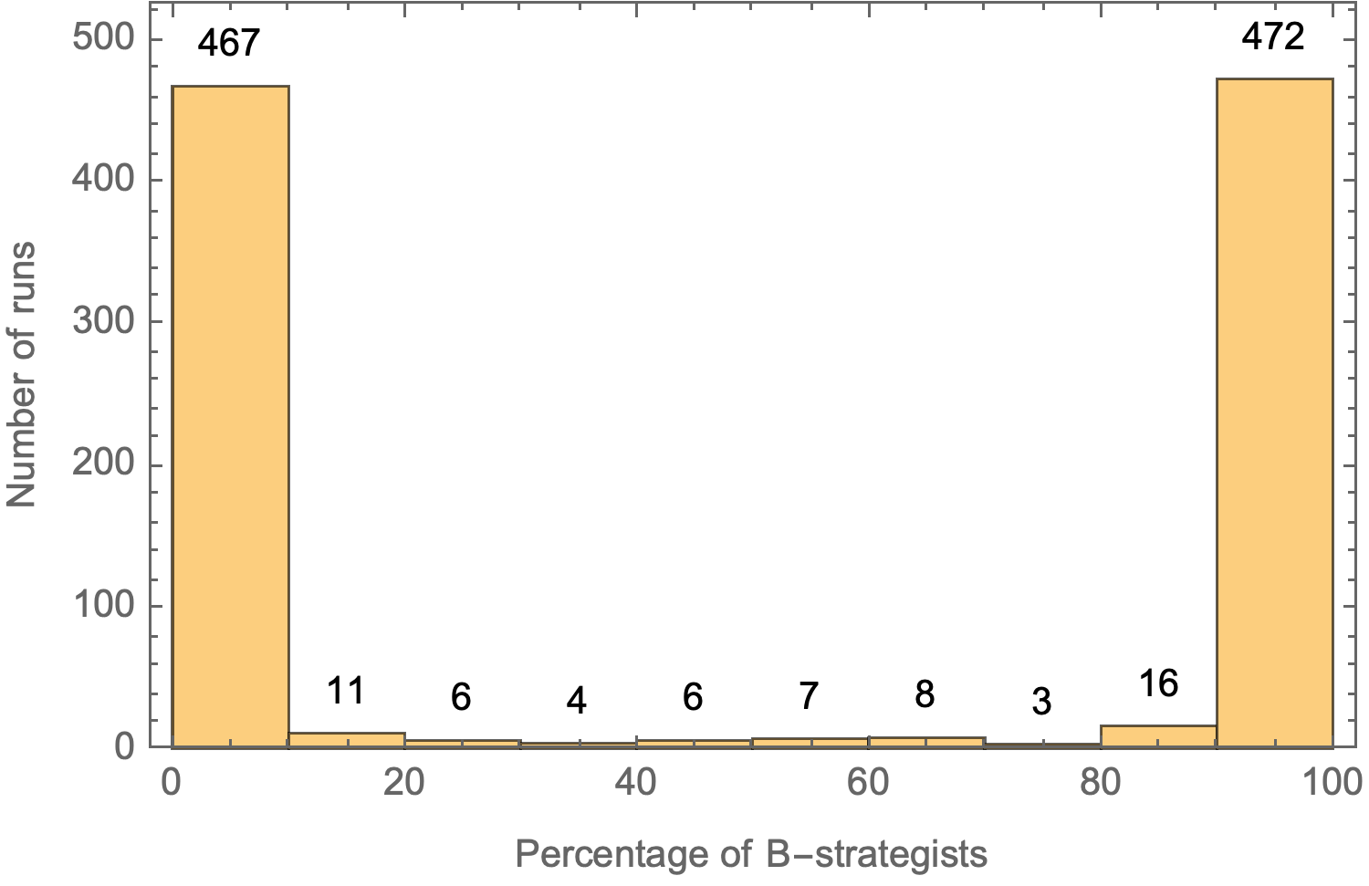
One point we would like to comment here is that we should try to report meaningful statistics. Some statistics can be deceiving in certain cases, and we should try to avoid them. For instance, reporting only the average of a bimodal distribution is not ideal, since the average masks the fact that the distribution is bimodal and may be easily misinterpreted.
We saw an example of a bimodal distribution in chapter IV-2. The 1000 simulations we ran there on a star network yielded an average percentage of B-strategists by tick 5000 equal to 50.33%. Looking at that average, one could (mistakenly) infer that, at tick 5000, roughly half the population uses strategy A and the other half uses strategy B. But actually, the truth is that the distribution is bimodal: in nearly half of the runs almost all agents were choosing strategy A, and in nearly half of the runs almost all agents were choosing strategy B (see figure 3 below).
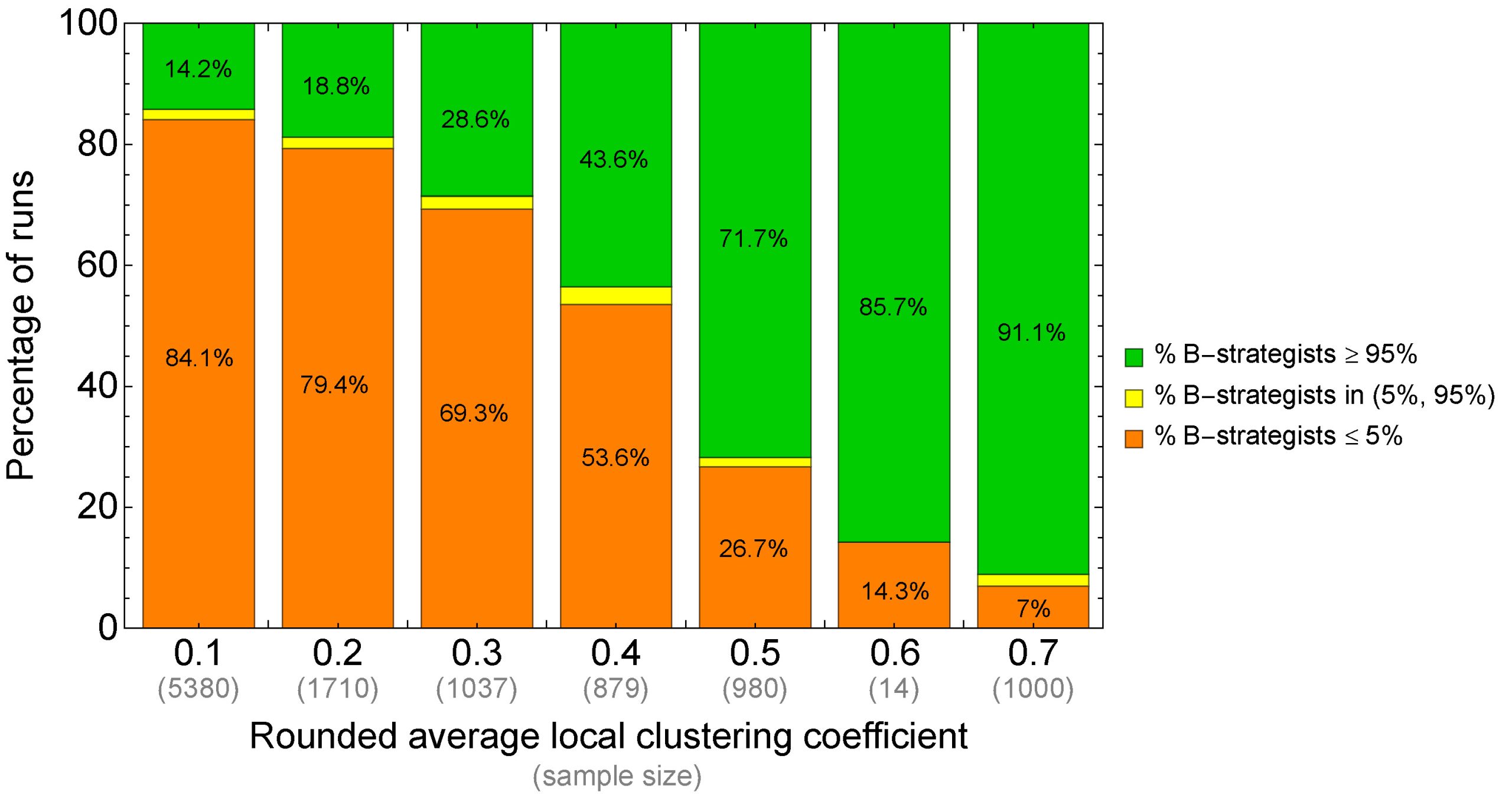
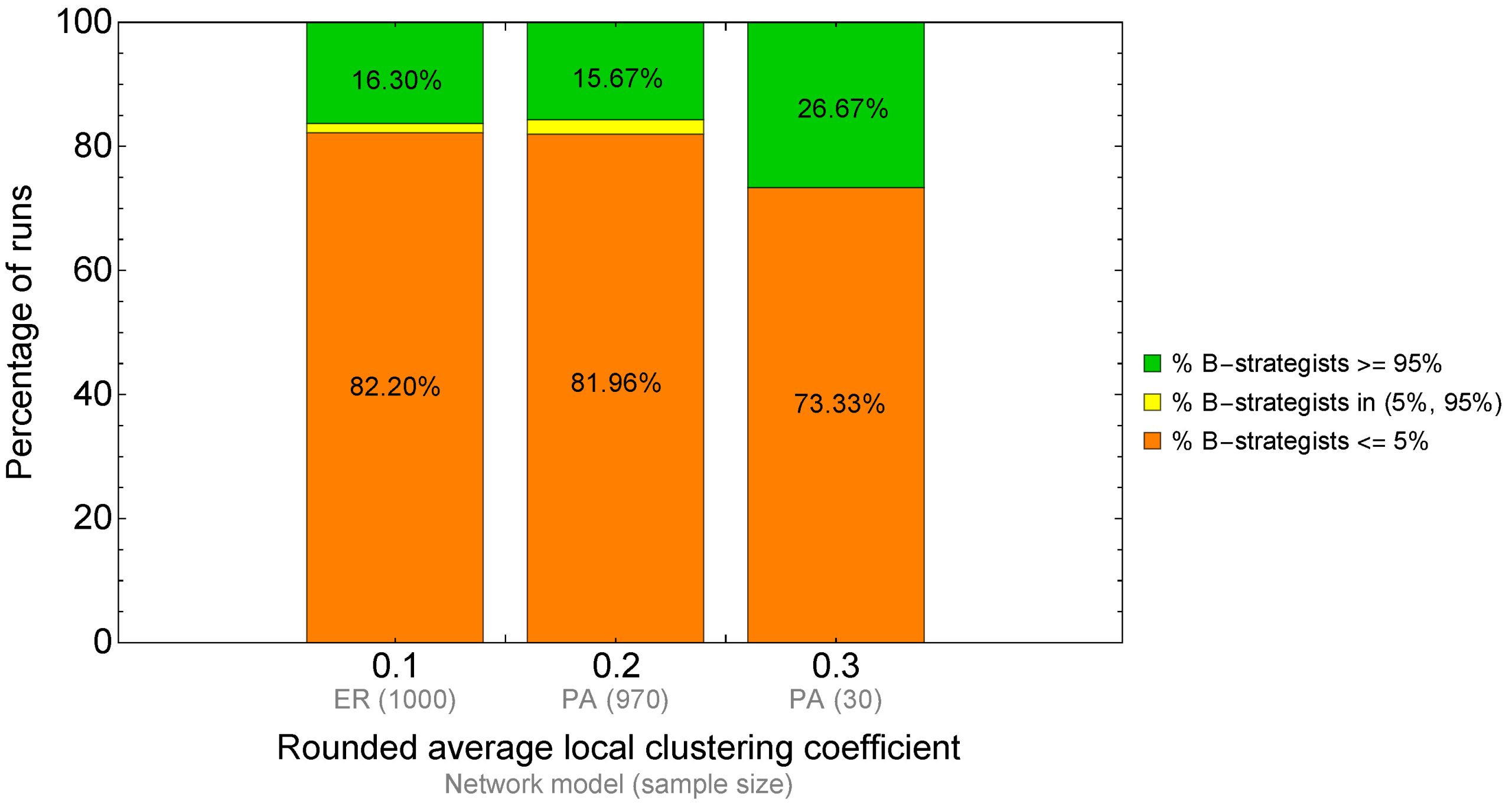
Multimodal distributions are very common in evolutionary models: these models tend to spend most of the time in one out of a small set of possible regimes. We saw another example of this feature in the sample runs of the previous chapter. The simulations we ran there spent most of the time at one of two possible regimes: one where the proportion of B-strategists was very high (≥ 95%) and another one where the proportion of B-strategists was very low (≤ 5%). Reporting only the average of B-strategists across runs would have been misleading in that case. It is more meaningful to report the percentage of runs that were at each of the two regimes, as we did in figure 7 and in figure 9.
5. Derive sound conclusions
Our goal when we analyze any model is to fully understand why we are observing what we are observing. In other words, we would like to identify the features or assumptions in our model that are responsible for the emergence of the phenomena we observe. To check whether a certain assumption is responsible for a particular phenomenon, we must be able to replace the assumption with an alternative one. Thus the importance of implementing and exploring various alternative assumptions (e.g. different decision rules, different ways of computing payoffs, different network-generating algorithms, etc.) to make sure that our conclusions are sound. If we don’t do this, we run the risk of over-extrapolating the scope of our model and even drawing unsound conclusions.
One feature that is often easy to implement and can provide important insights is noise. We have seen that the dynamics of many models can change significantly when we introduce small amounts of stochasticity in the agents’ behavior or in the way they revise their strategies (e.g., sequentially or simultaneously). We believe it is important to assess the robustness of any observed phenomenon to low levels of stochasticity since, after all, our models are imperfect abstractions of real-world systems that are usually significantly less deterministic and well-behaved.
6. Final thoughts
We realize that, after reading this chapter, you may feel overwhelmed by the amount of things that can go wrong when trying to draw sound conclusions using an agent-based model. You’re right: many things can go wrong. We hope that this book has opened your eyes in this respect but, more importantly, we hope that you have learned a wide range of useful techniques to avoid falling into the many traps that lie out there for the rigorous agent-based modeler. If you have managed to read this book until here, we are confident that you are now well prepared to implement and analyze your own agent-based models and to rigorously use these models to advance Science. It is also our hope that you will enjoy this process as much as we have enjoyed writing this book.
7. Exercises
![]() Exercise 1. Implement a procedure named to setup-players-special to create the network shown in figure 1.
Exercise 1. Implement a procedure named to setup-players-special to create the network shown in figure 1.

Exercise 2. Can you analytically derive the probabilities of reaching each of the end states shown in Table 1?
Exercise 3. Once you have implemented procedure to setup-players-special in exercise 1 above, design a computational experiment to estimate the exact probabilities shown in Table 1.
![]() Exercise 4. Imagine that you suspect that your model spends a significant amount of time in a regime where the proportion of players using strategy 1 is in the interval [0.3, 0.4]. Implement a reporter that returns 1 if the simulation is in this regime and 0 otherwise.
Exercise 4. Imagine that you suspect that your model spends a significant amount of time in a regime where the proportion of players using strategy 1 is in the interval [0.3, 0.4]. Implement a reporter that returns 1 if the simulation is in this regime and 0 otherwise.
![]() Exercise 5. Generalize the reporter you have implemented in Exercise 4 above so the endpoints of the interval (0.3 and 0.4 in exercise 4) are inputs that can be chosen by the user, and there are also two additional inputs to control whether each of the interval endpoints is included or excluded.
Exercise 5. Generalize the reporter you have implemented in Exercise 4 above so the endpoints of the interval (0.3 and 0.4 in exercise 4) are inputs that can be chosen by the user, and there are also two additional inputs to control whether each of the interval endpoints is included or excluded.
![]() Exercise 6. Once you have implemented the general reporter in Exercise 5, write the metrics you would have to include in BehaviorSpace to check whether the simulation is in each of the following regimes:
Exercise 6. Once you have implemented the general reporter in Exercise 5, write the metrics you would have to include in BehaviorSpace to check whether the simulation is in each of the following regimes:
- Proportion of players using strategy 1 is in the interval [0.3 , 0.4]
- Proportion of players using strategy 1 is in the interval (0.2 , 0.3]
- Proportion of players using strategy 1 is in the interval [0.6 , 0.8)
- Proportion of players using strategy 1 is in the interval [0.9 , 1]
- See Math section in NetLogo programming guide. ↵
- You may want to try this out in other programming languages such as Python, R, Javascript, Java, C, C++ ... ↵
- Number 3.6 is not exactly representable in binary, but since the result of 4 * 1 + 1 * (-0.4) is the closest floating-point number to 3.6, NetLogo outputs 3.6. ↵
- See also figure 5 (top left) in Tomassini et al. (2007). Tomassini et al. (2007) note that 10 000 ticks may not be enough for the metric to stabilize and run their simulations for much longer (21 000 ticks). They report a value above 30%, which is significantly higher than the one reported in Santos and Pacheco (2006). ↵
- For simplicity, we have computed the p-value ignoring ties (or, equivalently, assuming they are counted as success or failure with equal probability), using a simple two-tailed binomial test. In Mathematica:
↵
2 * CDF[BinomialDistribution[100, 0.5], 100 - 91]
