V-1. Introduction

Luis R. Izquierdo; Segismundo S. Izquierdo; William H. Sandholm

Part V. Agent-based models vs ODE models

V-1. Introduction

Many models in Evolutionary Game Theory are described as systems of Ordinary Differential Equations (ODEs). The most famous example is the Replicator Dynamics (Taylor and Jonker, 1978), which reads:

$\dot{x}_i = x_i (\pi_i - \pi)$

where:

$x_i$ is the fraction of $i$ -strategists in the population.
$\dot{x}_i = \frac{dx_i}{dt}$ describes how the fraction of $i$ -strategists $x_i$ changes in time.
$\pi_i$ is the expected payoff of strategy $i$ . That is, if $\pi_{ij}$ is the payoff that an $i$ -strategist obtains against a $j$ -strategist, then $\pi_i = \sum_{j} x_j \pi_{ij}$ . This is also the average payoff that an $i$ -strategist would obtain if he played with the whole population.
$\pi = \sum_{j} x_j \pi_j$ is the average payoff in the population.

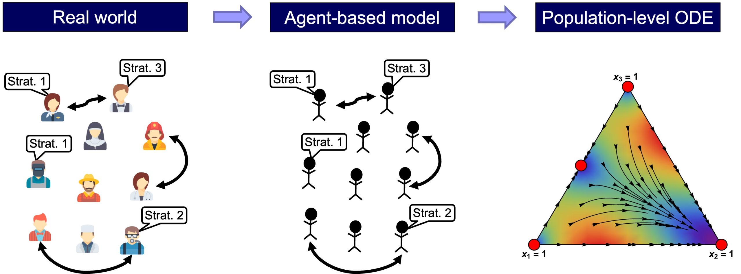
ODE models are very different from the agent-based models we have considered in this book. Our goal in this Part V is to clarify the relationship between these two kinds of models. We will see that most ODE models in Evolutionary Game Theory can be seen as the mean dynamic of an agent-based model where agents follow a certain decision rule in a well-mixed population.^[1] This implies that those ODE models provide a good deterministic approximation to the dynamics of the corresponding agent-based model over finite time spans when the number of agents is sufficiently large (Benaïm & Weibull, 2003; Sandholm, 2010a, chapter 10; Roth & Sandholm, 2013). For this reason, ODE models in Evolutionary Game Theory are often called infinite-population models (because they describe dynamics of populations whose size tends to infinity), while agent-based models are sometimes called finite-population models.^[2]

It is also clear that the ODE models represent a higher level of abstraction than the agent-based models, in the sense that the variables in the ODE models are population-level aggregates, while the agent-based models are defined at the individual level (fig. 1).

Figure. 1. Agent-based models are described at the individual level, while ODE models are described at the population level

In fact, in many cases, there is a wide range of different agent-based models which share the same mean dynamic. For instance, consider the replicator dynamics, which is often derived as the infinite-population limit of a certain model of biological evolution (see derivations in e.g. Weibull (1995, section 3.1.1), Vega-Redondo (2003, section 10.3.1) or Alexander (2023, section 3.2.1)). In the following chapters we will see that the replicator dynamics is also the mean dynamic of the following disparate agent-based models:^[3]

A model where agents in a well-mixed population follow the imitative pairwise-difference rule using expected payoffs (Helbing,1992; Schlag, 1998; Sandholm, 2010a, example 5.4.2; Sandholm, 2010b, example 1).
A model where agents in a well-mixed population play the game just once with a random agent and follow the imitative pairwise-difference rule (Izquierdo et al., 2019, example A.2).
A model where agents in a well-mixed population follow the so-called imitative linear-attraction rule using expected payoffs (Hofbauer, 1995a; Sandholm, 2010a, example 5.4.4; Sandholm, 2010b, example 1).
A model where agents in a well-mixed population play the game just once with a random agent and follow the so-called imitative linear-attraction rule (Izquierdo et al., 2019, remark A.3).
A model where agents in a well-mixed population follow the so-called imitative linear-dissatisfaction rule using expected payoffs (Weibull, 1995, section 4.4.1; Björnerstedt and Weibull, 1996; Sandholm, 2010a, example 5.4.3; Sandholm, 2010b, example 1).
A model where agents in a well-mixed population play the game just once with a random agent and follow the so-called imitative linear-dissatisfaction rule (Izquierdo et al., 2019, remark A.3).

In the next chapter, we extend the (well-mixed population) model we developed in Part II by including different decision rules that have been studied in the literature and different ways of computing payoffs. Then, in chapter V-3, we derive the mean dynamic of each of the possible parameterizations of this extended agent-based model. We will see that some parameterizations that generate different stochastic dynamics share the same mean dynamic. In this way, we hope that the (many-to-one) relationship between agent-based models and ODEs will be perfectly clear.

The term well-mixed population refers to a population where all individuals are equally likely to interact with each other. ↵
Another reason is that the fraction of $i$ -strategists $x_i$ in ODE models changes continuously in the interval [0,1], while in a finite population of $N$ individuals, this fraction would have to be a multiple of $1/N$ . See footnote 31 in Alexander (2023). ↵
Some of these models lead to the replicator dynamics up to a speed factor, i.e., a constant may appear multiplying the whole right-hand side of the equation of the replicator dynamics. This constant can be interpreted as a change of time scale. ↵

License

Icon for the Creative Commons Attribution 4.0 International License

Agent-Based Evolutionary Game Dynamics Copyright © 2024 by Luis R. Izquierdo, Segismundo S. Izquierdo & William H. Sandholm is licensed under a Creative Commons Attribution 4.0 International License, except where otherwise noted.

License

Share This Book