3 Lesson 3

Welcome to Lesson 3—Asking Spatial Questions and Modeling a Spatial Problem

In this lesson, you will:

• Be able to correctly identify the kind of spatial questions to ask, or being asked in a given problem
• Recognize considerations in planning a geographic information system (GIS) project, such as choosing data, toolsets, output needs, and ethical or error issues
• Select and use appropriate GIS tools to solve basic environmental spatial questions
• Identify a series of spatial questions and link them together logically (geoprocess thinking)
• Learn to build and run a basic geoprocessing model using ModelBuilder

1. Asking Spatial Questions

Despite what you may think, making maps is not the ultimate goal in your GIS education, at least not here. Watch this video by Kerski to see why:

https://youtu.be/qrHoVHq_Ag0

As Kerski said, our goal with GIS is to better understand our world and environment. To do so, we ask spatial questions about the parts of the world we are exploring. Here are the kinds of questions we can ask with GIS:

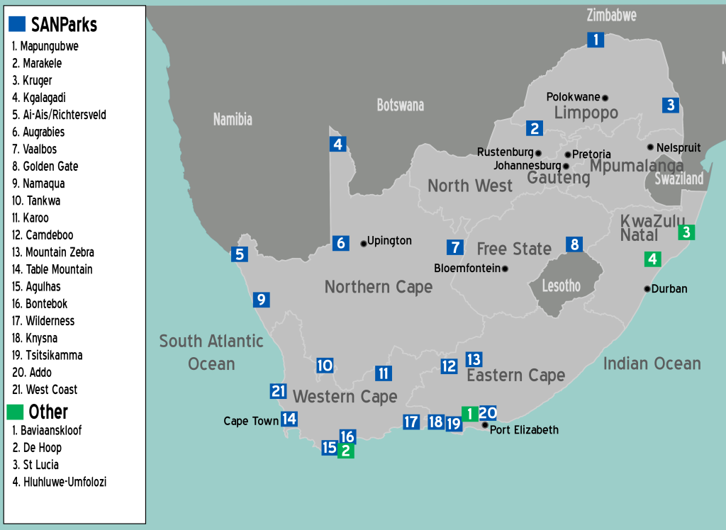
Location

Where is it? Find the location of all National Parks in South Africa.

Measurement

How far is it? Find the distance between Madison and Kettle Moraine State Park.

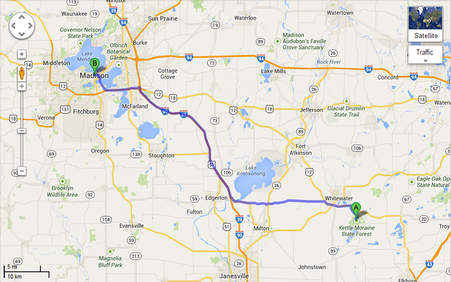
48.7 miles!

Condition

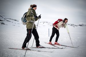
What location fits specific conditions? Find out which Ontario Parks have cross country skiing trails.

Proximity

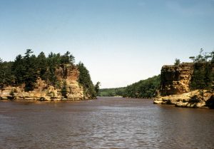
What is near it? Find out which Wisconsin State Parks are within 20 miles of the Wisconsin River.

Trends

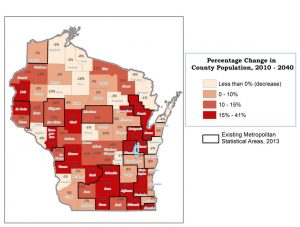
What has changed since...? Find out where Wisconsin’s population has changed since 1990.

Pattern

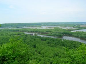
What spatial patterns exist? Find out if Wisconsin State Parks are clustered in certain regions such as the Driftless Area, or in areas of steep terrain.

Routing

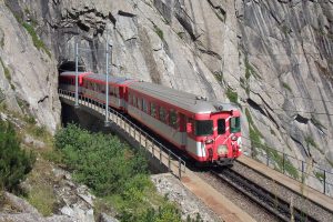
Which is the best way? Find the shortest route to the St. Gotthard Pass in the Swiss Alps.

Modeling

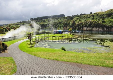
What if...? New Zealand wanted to create a new recreational park. Based on land cover, proximity to water, and characteristics most commonly sought by park visitors, where would be best location to create a new state park? What if specific features were prioritized differently—like proximity to an urban population?

Asking a Spatial Question

Asking a spatial question is the first step in GIS-based project planning. Often spatial questioning is an iterative process, where insights into the original question lead to additional, related questions that may be important to making informed decisions.

Carefully framing spatial questions will lead you to identify the best data to be gathered, explored, and analyzed. Often we have a great spatial dataset and try to frame questions around it so we can use GIS. Rather, it is more efficient to understand your spatial problem first, and then decide what tools and data you need to best solve it. It is really important to ask yourself, which data are most relevant to your questions, and to know when you have enough!

Then when selecting data for your project, you can use the data portals and metadata to consider the following:

• the original source, medium, format, and purpose of the data
• the projection, spatial and temporal resolution, and extent of the data
• the accuracy and reliability of the data
• the relevance of attributes to spatial question
• the accessibility and cost of the data

For a detailed list of considerations, see pages 238 and 239 of Kerski and Clark (2012).

Obtaining Spatial Data

Once we’ve determined our spatial question, we need to identify the spatial data we’ll need to answer or analyze our question.

As we covered in Lesson 2, sometimes, especially for more remote areas or unique spatial information, we may need to create and import our own spatial data.

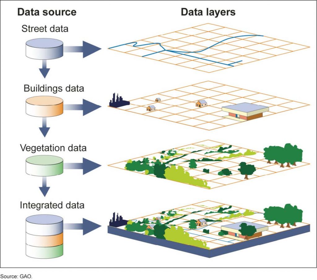
Very often though, existing data can fulfill the requirements. Acquiring public domain data can be much less time consuming and expensive than capturing new data.

Public domain data can be obtained from a variety of sources as we learned in Lesson 1, and do not always reside online. Geospatial one-stops and government or university map library collections provide access to a great deal of spatial data. Other offline and informal tools to locate relevant spatial data include the following:

• consulting the literature to find out which data similar studies or projects used
• contacting the data provider directly
• checking with local civic planning offices and community groups
• and grassroots mapping organizations like “Use-It”
  

  

Choice of Software

The spatial questions and data inform the choice of software to be used. Appropriate software, whether proprietary (e.g., ArcGIS) or open source (e.g., QGIS), will:

• enable you to work with the data input for the project
• have the needed display and analytical functionality
• provide appropriate access (sharing), or not (security)
• support the output formats necessary to generate required end products
• fit the project’s budget
• be accompanied by the appropriate level of user support

Both the spatial question and choice of software will help determine who will carry out data acquisition, analysis, and delivery of final products. Careful planning at each of these steps will help balance efforts toward data acquisition with those toward data analysis.

 

Topic 1 Knowledge Check

2. Geoprocess Thinking

Geoprocessing

Now we will dig into spatial thinking a little deeper. Geoprocessing refers to a framework, tool, or set of functions to query and manipulate spatial data. Geoprocessing allows for spatial data questions or problems to be addressed. Let us see how:

Basically, one or more input spatial datasets goes through a single geoprocessing tool, resulting in a new transformed output layer. Individually these tools perform small but necessary steps, such as “buffer” or “select feature” to move your spatial data from one form to another.

 

 

 

We can link a series of geoprocessing tools together and save the process to run it over and over again with different input data or parameters.

Chaining together a series of spatial data and geoprocessing tools creates a geoprocessing model, where the output of one step feeds the input for the next function. Geoprocess models become incredibly useful when working with multiple data layers (e.g., a time sequence of land cover) to analyze complex spatial relationships and reveal new insights. And, they can even be automated to run iterations with batch input or parameters. For example, a geoprocess model could be used to identify areas most prone to landslides over time in a developing area by inputting a time series of development maps and iteratively changing the slope criteria to see how the output areas change.

Geoprocessing Examples

Lets take a look at a few examples of geoprocessing applications.

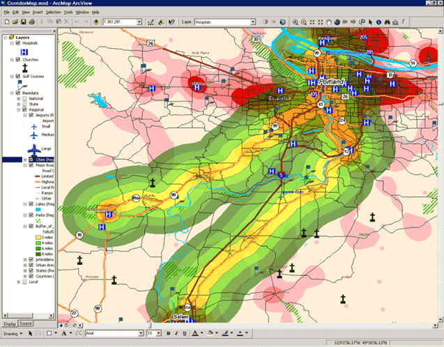
Locating a Pipeline Corridor or Landfill

Spatial Question: What areas would be in some proximity of a proposed pipeline and could be affected by it?

Use the buffer tool to select the area within a chosen distance of the proposed pipeline pathway to identify ecologically and socially vulnerable areas and understand environmental justice implications.

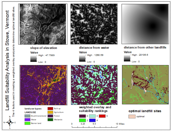
Spatial Question: What areas meet certain conditions identified as important for the location of a new landfill?

To identify the suitable locations for a landfill, use the overlay tool to identify locations in which slope, distance from water and other landfills, and certain land use types coincide.

• Each criteria must be carefully selected
• Decide if each receives equal weight. If not, which gets more? How much more?
• Think about any uncertainty in these criteria and how that might affect decisions for park placement

Recommended Fertilizer Application

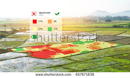
Spatial Question: A farmer has a limited amount of fertilizer for her hops crop. Where should she apply it?

Determine the spatial pattern of soil nutrient deficiency by mapping soil nutrient data and selecting by area where nutrient availability, for example, potassium (K), is lower than the minimum recommended levels for her crop of hops.

Geoprocessing Operations

In each of the previous examples, geoprocessing operations were performed in specific sequences to answer the question from the available input data.

Specifically, geoprocessing tools take input spatial data, perform a specific operation on those data, and return the result as an output dataset. For instance, you might have two input layers which you “intersect” in geoprocessing to return a single output layer.

Often operations may focus on selecting areas that fit specific criteria, such as selecting for certain attributes, clipping to a boundary, or defining a proximity. You will learn more about specific geoprocessing operations in Topic 3. First, there are some considerations for geoprocessing . . .

Accuracy

When we start combining different spatial data in geoprocessing operations, inaccuracies in the input layers can impact the output. Recall that the accuracy of spatial data is the fidelity with which the data represent real-world phenomena. Accuracy of spatial data can be reduced by:

• Measurement error
• Projection distortion
• Abstraction of real-world objects
• Generalization
• Classification
• Natural variability

Therefore, when combined, the error of each input dataset propagates to the output data.

Addressing Uncertainty

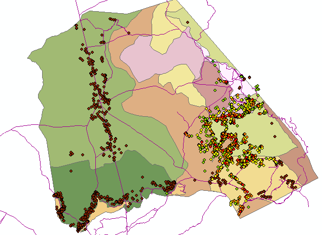
Due to the inevitable inaccuracy of input data, the output data resulting from geoprocessing operations are inherently uncertain. Therefore, geoprocessing operations ideally should consider OR quantify uncertainty to assess the effect on the resulting conclusions.

If data are not accurate, errors are propagated and the uncertainty grows with each geoprocessing step, which affects the accuracy of the results.

Sensitivity Analysis

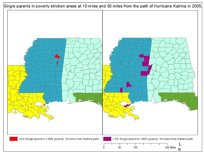
To evaluate uncertainty and explore what happens from your geoprocessing steps, a sensitivity analysis is recommended. Sensitivity analyses simply run multiple iterations of the same geoprocessing steps using different variables to investigate how a process and resulting output respond to changes in input information.

For example, changing the slope criteria from 0%–5% to 0%–10% in a site suitability model, or the buffer distance from a hurricane path in a vulnerability model might lead to very different suitable/vulnerable areas in the output.

Sensitivity analyses help us understand the relationships between input and output, estimate how much variability the model produces for each change in the inputs, and identifies which input source contributes most strongly to the output.

The following scenario illustrates how spatial questioning, geoprocess thinking, and sensitivity analysis are combined to inform decision-making.

Gnatcatcher Habitat Suitability

A local land trust wishes to protect habitat for the gnatcatcher, a bird of conservation concern. To do so, they undertake the following activities:

• Formulate a Spatial Question
• Summarize Habitat Requirements
• Obtain Spatial Data
• Geoprocessing
• Sensitivity Analysis

And this is what they know about the bird:

Gnatcatchers live in coastal sage scrub less than 228m asl (above sea level) in patches greater than 10 hectares. They have been shown to be sensitive to roads, and will not nest in areas with a slope greater than 40%.

Formulate a Spatial Question

Where are areas of suitable gnatcatcher habitat located?

Summarize Habitat Requirements

Cover type: Coastal sage scrub

Minimum patch size: 10 hectares

Elevation: Less than 228m asl

Excludes areas within 250m and 400m of roads

Obtain Spatial Data

• Land cover map
• Road map
• Digital elevation model (DEM) or triangulated irregular network (TIN) (elevation)

Geoprocessing

The Land Trust team starts with a sketch to plan the sequence of geoprocessing operations necessary to integrate and analyze the data to inform the spatial question. Although it can be tempting not to sketch or diagram your steps first, doing so allows the question to drive the process, not the tools.

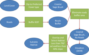
Then the team uses GIS software to perform the geoprocessing.

Geoprocessing will result in a map showing the location of habitat suitable for gnatcatchers, according to your process.

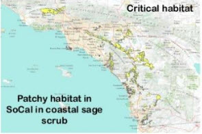
Sensitivity Analysis

Now, what if you are not sure whether your model best represents actual gnatcatcher habitat. Several parameters could be explored to test the sensitivity of the model, including:

• Reducing max permissible slope from 40% to 30%, 25%, and even 20%. Is most of the available habitat lost when areas with a slope between 40% and 30% are eliminated? How does this affect the decision to protect specific areas?
• Increase or decrease buffer around roads or use a more detailed road layer. Does a larger or smaller buffer or greater number of roads dramatically influence the total habitat area?
• Include cat population density. Do areas of suitable habitat coincide with areas of high cat population density? How does this influence the choice of specific areas?

Topic 2 Knowledge Check

3. Using ModelBuilder

Now let us get our hands dirty and learn how to apply geoprocessing within GIS by opening the toolbox . . .

Geoprocessing operations in GIS are carried out using a set of tools, organized into toolsets, each of which performs a single operation.

• Data Extraction
• Overlay
• Proximity

Data Extraction

There are several methods available to reduce or extract data from larger, more complex datasets to create a new subset of data with just the information needed.

Selection tools—allow you to select features that meet some criteria or that are located in a particular place, or a combination of both, such as “all the non-vacant parcels adjacent to the parkway” (below).

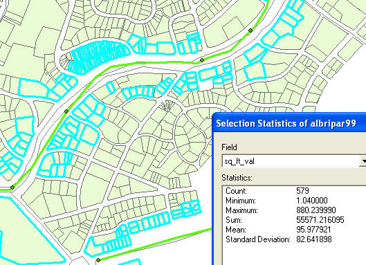
Other basic spatially defined selection tools include the following:

• Clipping—works like a cookie cutter to cut out features from the input layer that fall within the polygons in the clip feature
• Splitting—creates multiple output layers from a single feature layer based on polygons or zones of the split features
• Dissolving—combines polygons that share an attribute value into larger polygons, essentially dissolving the border between the features
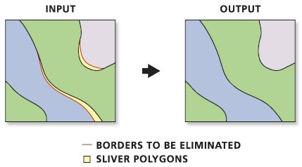
• Eliminating—combines selected polygons with adjacent polygons that have the largest area or longest shared border. Eliminate is often used to clean up spatial data after digitizing or overlaying features by eliminating sliver polygons

Dissolving and eliminating features can be used to extract features that share particular attributes, and combine them into larger features with less diversity

Dissolve

Eliminate

Overlay

Spatial Overlay

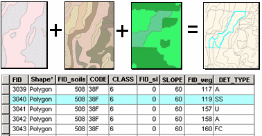
Spatial overlay superimposes multiple datasets with a common coordinate system, resulting in a new dataset that identifies the spatial relationships between multiple data layers.

Vector Overlays

Vector overlays are created when a polygon layer is placed over a feature layer containing points, lines, and/or polygons. Vector overlays can be accomplished using several tools, including identity, intersect, union, symmetrical difference, and update.

Below is an example of an overlay of steep slopes, soils, and vegetation. New polygons are created by the intersection of the input polygon boundaries. The resulting polygons have all the attributes of the original polygons.

Raster Overlay

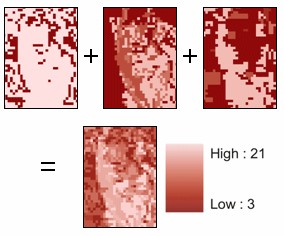
Raster overlay mathematically merges two or more sets of data that share a common grid to create a new set of values for a single output layer. Raster overlay tools include combine, zonal statistics, map algebra, weighted overlay, and weighted sum.

Below is an example of raster overlay by addition for suitability modeling. Three raster layers (steep slopes, soils, and vegetation) are ranked for development suitability on a scale of 1–7. When the layers are added (bottom), each cell is ranked on a scale of 3–21.

Proximity

Proximity tools find the distance of cells or proximity of features to one another and operate differently depending on the input data model.

Vector Proximity Tools

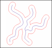
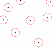
Vector proximity tools include buffer, near, point distance, select by location, and others. The images below illustrate a line (left) and point (right) buffer.

Raster Distance Tools

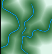
Raster distance tools include Euclidean distance, Euclidean direction, cost distance, cost allocation, and others. The image below illustrates output of the Euclidean Distance tool, where the value of each cell is the distance to the nearest river feature.

Using ModelBuilder

There are several ways to spatially select portions of a data layer. 

Set Algebra

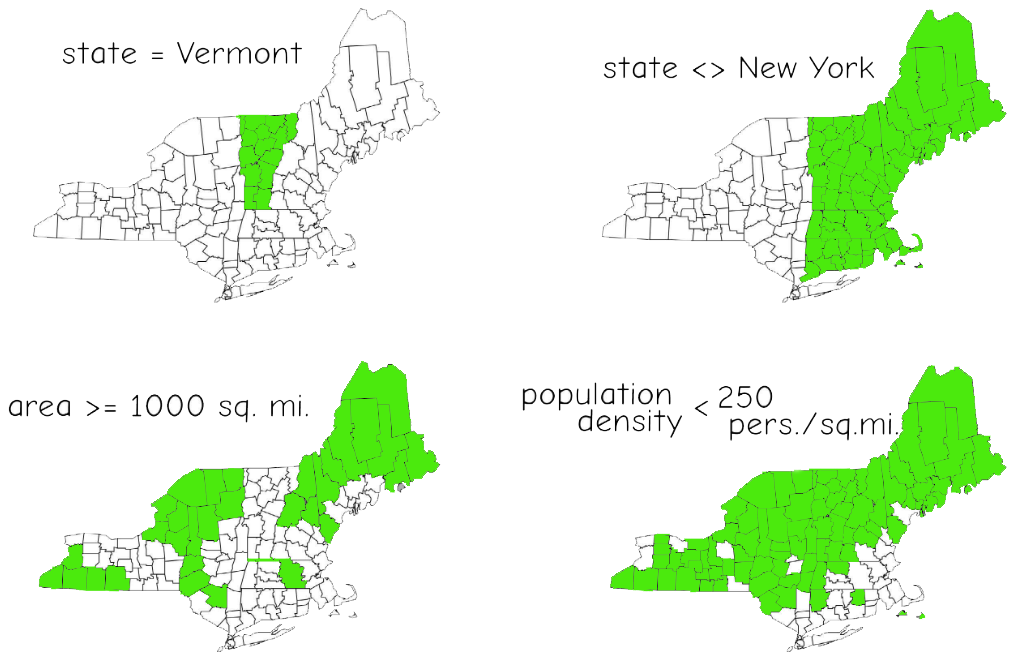
Remember learning what fit in a set in elementary algebra? Set algebra chooses areas with attributes that are >, <, or = to some specified criteria.

For example, you could select all areas that are not “New York” (upper right), or all counties that are at least 1000 square miles in area (lower left):

Boolean Operations

Similar to Set Algebra, Boolean algebra chooses areas with attributes matching specified criteria using AND, OR, NOT operations.

Fuzzy Set

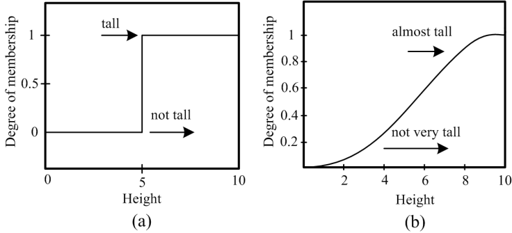
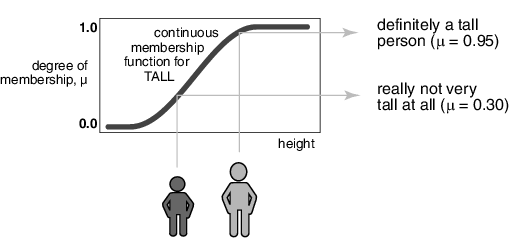
Fuzzy selection is less commonly used in GIS than other selection sets. When attribute data are imprecise or inaccurate, fuzzy logic can be used to define how likely it is that a particular feature or cell is a member of a set. In the example below, fuzzy sets are used to identify the likelihood that an individual will fall into the “tall” class. You might also imagine this applied to environmental features, like the probability that energy sites will have high radon levels. We will come back to fuzzy logic more later.

Geoprocess Functions

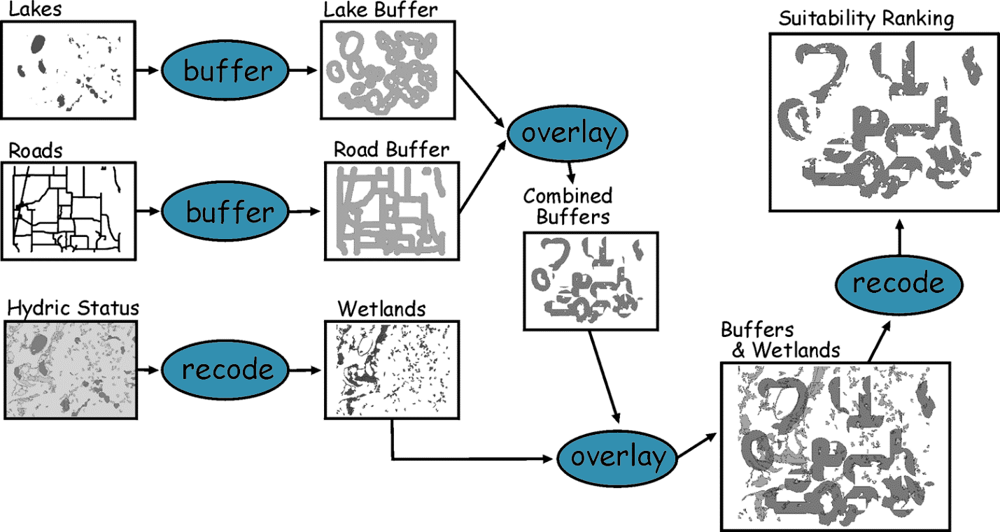
Geoprocessing tools can be linked together to perform a series of operations necessary to produce the output that answers a spatial question. Each step produces intermediate output on which the next operation acts.

In the example below, buffers are created around the lakes and roads in their respective layers and then overlaid to eliminate areas where roads intersect lake buffers. The hydric status layer is recoded to identify wetlands. Then the wetlands layer and combined buffers layer are overlaid, and areas where the lake buffer and wetland buffer coincide are recoded with a suitability ranking.

Geoprocess Demo

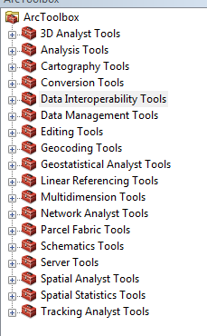
In ArcGIS, geoprocessing tools are accessible from ArcToolbox and ArcCatalog and are stored in toolsets, which are stored in toolboxes. Please click here to watch a YouTube demonstration of the use of ArcToolbox in ArcMap 10. The video is approximately 11 minutes long.

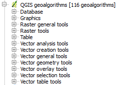
Here you see how geoprocessing tools are organized in ArcToolbox of ArcGIS (left) and the Geoalgorithms Toolbox in QGIS (right):

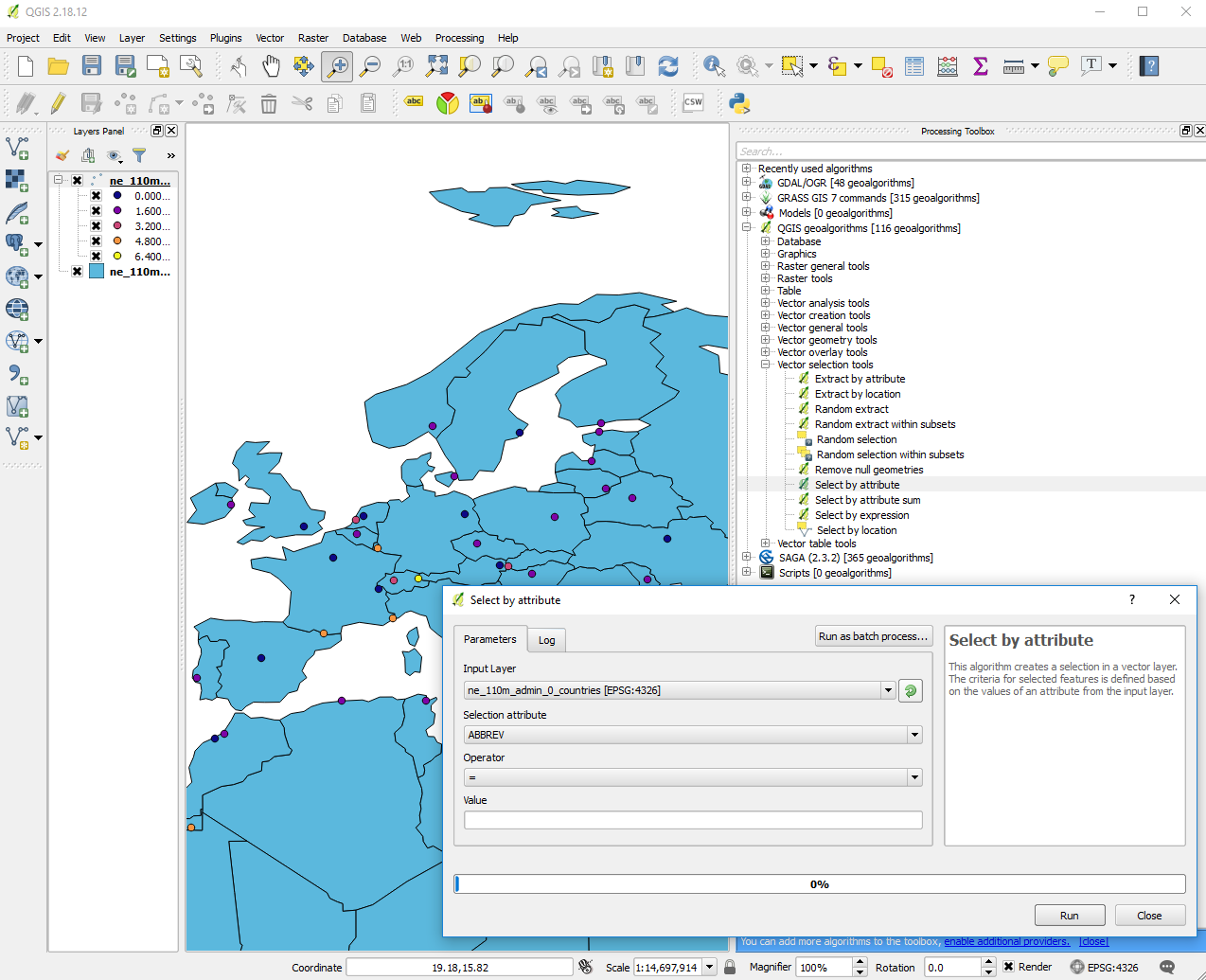
Below shows a geoprocessing tool pop-up window accessed from the toolbar on the right in QGIS:

Geoprocess Model Design

Geoprocessing sequences are also referred to as a “model.” Consider these typical steps in designing your first geoprocessing model:

• Determine which geoprocessing tools you need (based on your spatial question).
• Have your spatial data prepared and organized in Catalog.
• Determine the order in which the geoprocessing tools should be used.
• Locate the first tool and open its dialog box.
• Enter the tool parameters, including the input and output datasets.
• Run the tool.
• Repeat steps 3–5 for each geoprocessing tool. Rearrange as needed.
• Examine the final output and repeat some or all of the analysis steps as needed.

ModelBuilder

A model is a collection of geoprocessing operations that automatically execute in sequence when the model is run to produce a final output dataset. These can be put together using ModelBuilder in ArcGIS, or Graphical Modeler in QGIS. Any geoprocessing operation in a model can be modified, and then the model can be run again to quickly refine an analysis or produce new data that support an alternative (“what if?”) scenario.

Geoprocessing models are often used . . .

• For linking and automating analyses
• To document the flow through the processes of a project
• To modify inputs and processes easily in a graphic environment (e.g., to run a sensitivity analysis)
• To automate a repetitive process (e.g., multiple scenarios) to save time and effort.

For more, see this page on ArcGIS Desktop Analytics.

http://www.qgistutorials.com/en/docs/processing_graphical_modeler.html

Link to QGIS documentation on the graphical modeler: https://docs.qgis.org/2.18/en/docs/user_manual/processing/modeler.html?highlight=graphical%20modeler

Topic 3 Knowledge Check

Please answer the following questions to complete Lesson 3 (note: click the + sign to enlarge graphics).

References

Bolstad, Paul. 2016. GIS Fundamentals. 5th ed. XanEdu Press, http://www.paulbolstad.net/gisbook.html

Kerski, Joseph J. and Jill Clark. 2012. The GIS Guide to Public Domain Data. Esri Press, Redlands, CA 372 pp. Chapter 7 accompanies this lesson.

Moradlou, Majid, Farzaneh Eshaghian Dorcheh, and Mehdi Bigdeli. 2013. “Application of Superposition and Fuzzy Logic Methods to Determine the Contribution of the Utility and Customer in Creation of Harmonic Distortions in PCC Bus.” International Journal of Energy Engineering 3 (3): 138–46.