
Part I. Introduction
I-1. Overview
1. What is this book about?
This book is a guide to implement and analyze Agent-Based Models within the framework of Evolutionary Game Theory, using a programming language called NetLogo.
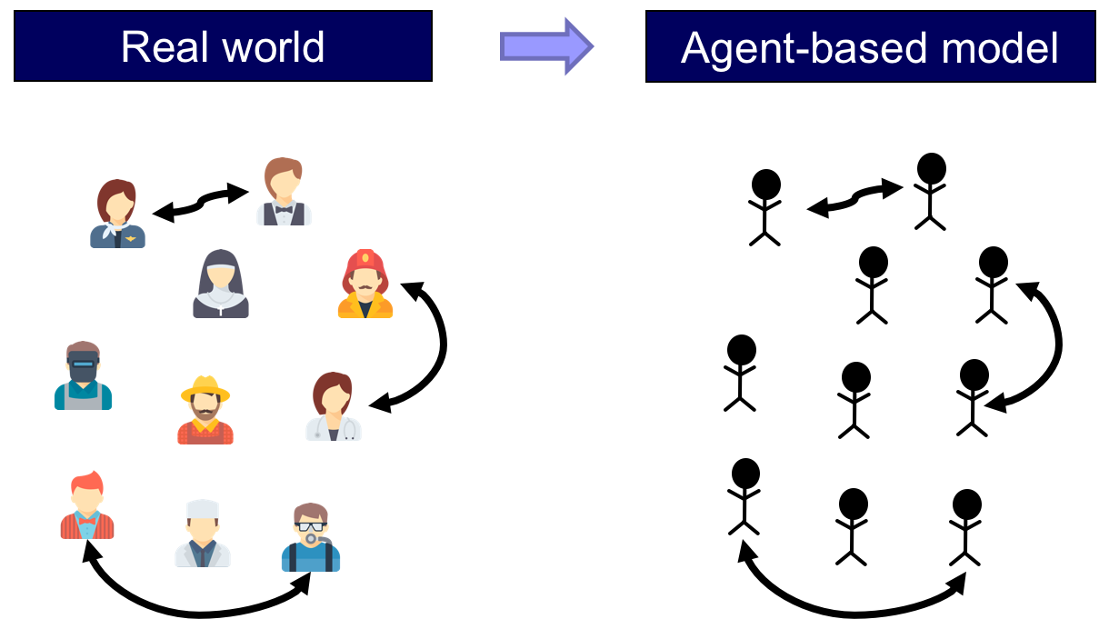
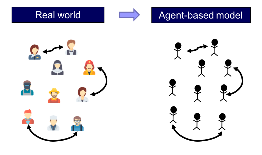
Let us flesh out the main terms in the previous sentence. A model is an abstraction of the real world and, basically, agent-based models are models where individuals and their interactions are explicitly represented in the model (see fig. 1).
Agent-based models are most often implemented as computer programs, and the programming language we are going to use in this book is NetLogo. And finally, game theory is a formal theory devoted to studying interactions among individuals whose actions affect each other. In particular, evolutionary game theory studies populations of individuals who may change their actions in time.
In this book we are going to learn how to implement agent-based models in NetLogo, within the framework of evolutionary game theory, and we are also going to learn how to analyze these models using both computer simulation and mathematical analysis.
2. How is this book organized?
The book is divided into five parts:
Structure of the book
- Part I. Introduction
- Part II. Our first agent-based evolutionary model
- Part III. Spatial interactions on a grid
- Part IV. Games on networks
- Part V. Agent-based models vs ODE models
Each part contains several chapters; and each chapter corresponds to one webpage in the online webbook.
The following sections summarize each of the parts of the book. To do this, admittedly, we will have to use concepts that you may not be familiar with, just yet. Apologies for that, but do not worry. We will define and explain every concept we use here in the following chapters.
2.1. Part I. Introduction
This first part contains the following chapters:
Part I. Introduction
- Chapter I-1. Overview
- Chapter I-2. Introduction to evolutionary game theory
- Chapter I-3. Introduction to agent-based modeling
- Chapter I-4. Introduction to NetLogo
- Chapter I-5. The fundamentals of NetLogo
This very chapter you are now reading is “Chapter I-1. Overview”. The rest of the chapters in this first part are introductions to the three main components of the book: evolutionary game theory (chapter I-2), agent-based modeling (chapter I-3), and NetLogo (chapter I-4 describes the main features of NetLogo, while chapter I-5 is a tutorial on programming in NetLogo). These introductions are self-contained and independent, so if you are already familiar with any of these topics, feel free to skip the corresponding chapters.
2.2. Part II. Our first agent-based evolutionary model
In Part II we implement our first agent-based evolutionary model, which is a simple model of a well-mixed population. The term well-mixed population refers to a population where all individuals are equally likely to interact with each other. Part II includes the following chapters:
Part II. Our first agent-based evolutionary model
- II-1. Our very first model
- II-2. Extension to any number of strategies
- II-3. Noise and initial conditions
- II-4. Interactivity and efficiency
- II-5. Analysis of these models
- II-6. Answers to exercises
In chapter II-1, we implement a model where agents repeatedly play a symmetric 2-player 2-strategy game (chosen by the user) and follow a simple rule to update their strategies. The code for this first (fully-functional) model fits in one page. In chapter II-2 we extend this model to allow for games with any number of strategies. Then, in chapter II-3, we add two very useful features to the model: the possibility of setting initial conditions explicitly, and the possibility that revising agents select their strategy at random with a small probability (i.e., noise). In chapter II-4, we improve the interactivity of our model (i.e., the possibility of changing the value of parameters at runtime, with immediate effect on the dynamics of the model) and its efficiency (i.e., we modify the code of our model to make it run significantly faster).
Chapter II-5 does not extend the model anymore. Instead, this chapter focuses on how to analyze it using both computer simulation and mathematical analysis. In this chapter, we present different mathematical theories and approximations that can be used to analyze agent-based evolutionary models of well-mixed populations. In particular, we discuss the theory of Markov chains and we introduce various mathematical techniques such as the mean dynamic, the diffusion approximation and stochastic stability analyses.
Finally, in chapter II-6, we provide the solution to the 30 exercises proposed in this part.
2.3. Part III. Spatial interactions on a grid
Part III is self-contained and completely independent of Part II. In Part III, we show how to build and analyze agent-based models with spatial structure. The video below shows an illustrative run of a population of agents embedded on a 81×81 spatial grid. Each cell represents an agent. Agents play a game called the Prisoner’s Dilemma with their neighbors. In the video below, agents are colored according to their current strategy and their previous one.[1]
In the models implemented in this part, agents do not interact with other agents with the same probability (as in Part II), but they interact only with those who are nearby in space. Populations where not every agent is equally likely to interact with each other are called structured populations (as opposed to well-mixed populations). Part III includes the following chapters:
Part III. Spatial interactions on a grid
- III-1. Spatial chaos in the Prisoner’s Dilemma
- III-2. Robustness and fragility
- III-3. Extension to any number of strategies
- III-4. Other types of neighborhoods and other decision rules
- III-5. Analysis of these models
- III-6. Answers to exercises
In chapter III-1, we implement a model where agents embedded on a grid repeatedly play a symmetric 2-player 2-strategy game (chosen by the user) with their spatial neighbors. The code for this first spatial model can perfectly fit in one page. In chapter III-2, we add three very useful features to the basic spatial model: noise, asynchronous strategy updating, and the possibility to choose whether agents play the game with themselves or not. We use these features to assess the robustness of various results in the literature. Then, in chapter III-3, we extend the model to allow for games with any number of strategies. In chapter III-4, we add two features that are crucial to assess the impact of space on evolutionary dynamics: the possibility to model different types of neighborhoods of arbitrary size, and the possibility to model different decision rules agents may use to update their strategy. The resulting model allows us to replicate many results in the literature.
Chapter III-5 does not extend the model anymore, but instead focuses on how to analyze it using both computer simulation and mathematical analysis. In this chapter, we explain what cellular automata are, and we discuss the pair approximation, a mathematical technique that is sometimes used to approximate the dynamics of evolutionary models on grids.
Finally, in chapter III-6, we provide the solution to the 29 exercises proposed in this part.
2.4. Part IV. Games on networks
In Part IV, we show how to implement and analyze agent-based models where players are connected through a network (fig. 2). In our models, the nodes in the network are the players, and each link connects two players.

In network models, we assume that players can only interact with their link-neighbors (i.e. those with whom the player shares a link), so link-neighbors are the only players that a player can observe or play with.
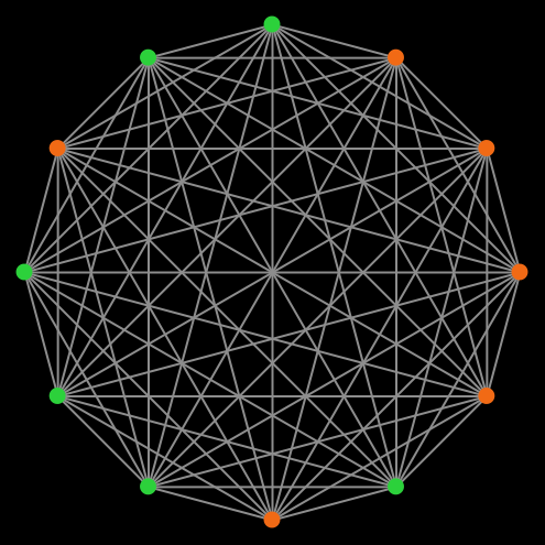
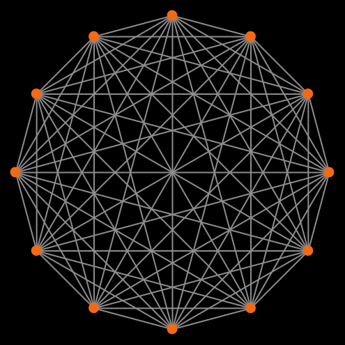
By using networks, we are able to generalize all the models previously developed in the book. Note that in Part II we implement models where every player could observe and play with every other player. Such models can be interpreted as network models where players are connected through a complete network, i.e., a network where everyone is linked to everybody else (fig. 3).
The spatial models developed in Part III can also be interpreted as network models. For instance, a grid model where adjacent cells (i.e., players) are neighbors (fig. 4a) corresponds to a square lattice network (fig. 4b).
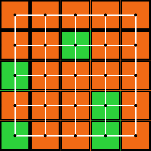
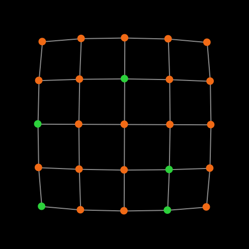
Figure 4. (a) A grid model where adjacent cells are neighbors and (b) an equivalent representation as a square lattice network
In this Part IV, we learn to implement models where players are connected through any arbitrary network. Part IV includes the following chapters:
Part IV. Games on networks
- IV-1. The nxn game on a random network
- IV-2. Different types of networks
- IV-3. Implementing network metrics
- IV-4. Other ways of computing payoffs and other decision rules
- IV-5. Analysis of these models
- IV-6. Answers to exercises
In chapter IV-1, we modify the well-mixed population model implemented in Part II by embedding the players on a random network. In chapter IV-2, we extend our random-network model by adding the possibility of creating many other types of networks, such as small-world, preferential attachment, rings, stars, wheels, paths, etc. This allows us to assess the significance of network structure on evolutionary dynamics. Then, in chapter IV-3, we implement several functions to compute network metrics such as the density, the size of the largest component, the clustering coefficient and the degree distribution. Chapter IV-4 greatly generalizes the model by adding two features that can have a major impact on evolutionary dynamics on networks: the possibility to model different ways of computing payoffs and the possibility to model different decision rules that agents may use to update their strategy. With this final network model we are able to replicate and discuss many results in the literature.
Chapter IV-5 does not extend the model anymore. Instead, this chapter focuses on how to analyze it. In this chapter, we discuss four best practices that can help us to analyze evolutionary dynamics using computer simulation.
Finally, in chapter IV-6, we provide the solution to the 30 exercises proposed in this part.
2.5. Part V. Agent-based models vs ODE (Ordinary Differential Equation) models
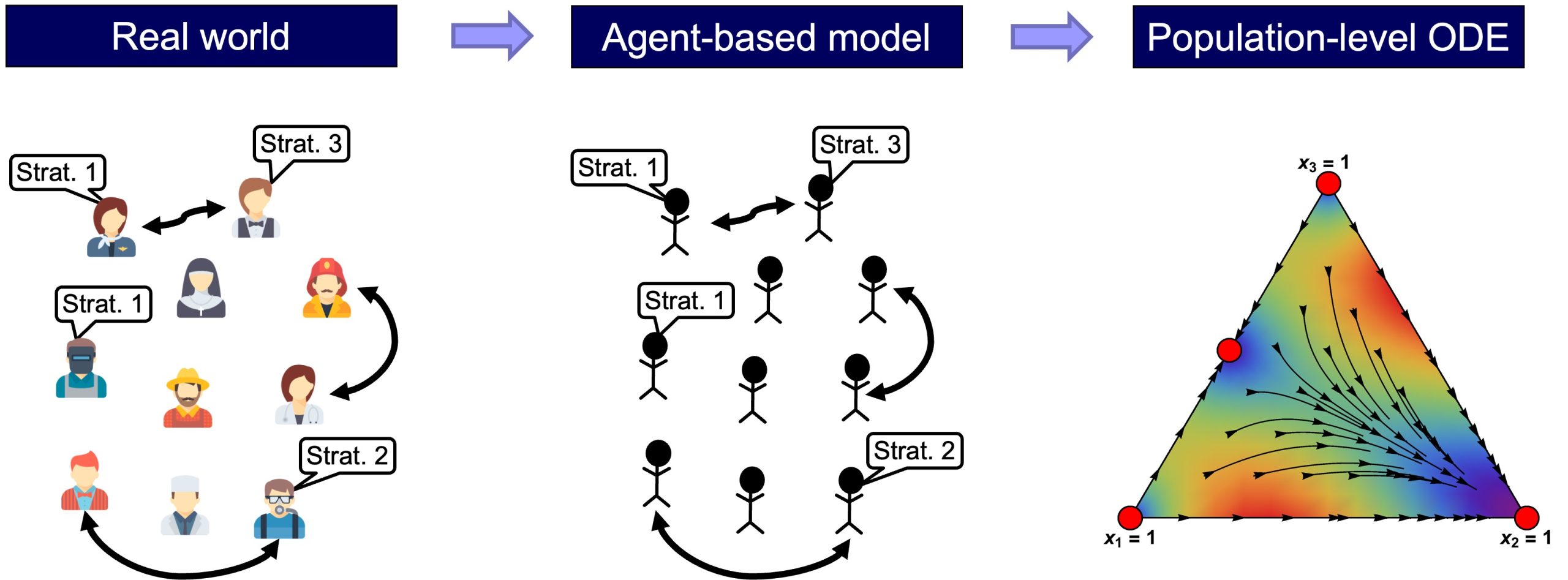
Many models in the Evolutionary Game Theory literature are described as systems of Ordinary Differential Equations (ODEs). The most famous example is the Replicator Dynamics (Taylor and Jonker, 1978). These mathematical models are very different from the agent-based models we consider in this book. Our goal in Part V is to explain the relationship between these two kinds of models. We will see that ODE models in the literature can be seen as approximations to the dynamics of different agent-based models when the population is large (fig. 5).
Part V includes the following chapters:
Part V. Agent-based models vs ODE models
- V-1. Introduction
- V-2. A rather general model for games played in well-mixed populations
- V-3. Mean Dynamics
- V-4. Answers to exercises
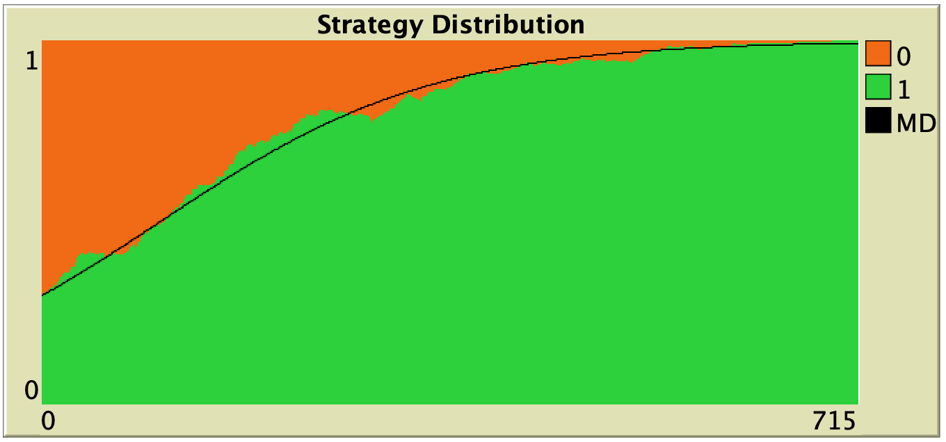
Chapter V-1 provides an introduction to the (many-to-one) relationship between agent-based models and ODE models. In chapter V-2, we generalize the well-mixed population model implemented in Part II by adding two important features: the possibility to model different ways of computing payoffs and the possibility to model different decision rules that agents may use to update their strategy. Then, in chapter V-3, we derive an ODE approximation (i.e., the mean dynamic) for every possible parameterization of our new (and fairly general) agent-based model. In this chapter we also learn how to numerically solve ODEs within NetLogo at runtime. This functionality allows us to compare agent-based simulations and their ODE approximations at runtime (fig. 6).
Finally, in chapter V-4, we provide the solution to the 12 exercises proposed in this part.
2.6. Appendices
The book contains three appendices:
- In Appendix A-1, we explain that oftentimes there are different ways of implementing any particular model, and we comment on how to choose the most appropriate implementation for a given purpose.
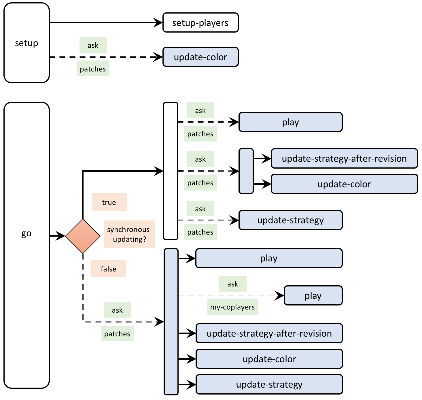
- The book contains many code skeletons that provide a schematic bird’s-eye view of the code. Figure 7 below shows an example. Appendix A-2 includes the legend to interpret these code skeletons.
- Finally, Appendix A-3 includes links to download each of the 22 NetLogo programs that are implemented in this book.
- The settings for this simulation run are defined in the Discussion section of chapter III-2. ↵
