2.4. Analysis of these models

Luis R. Izquierdo; Segismundo S. Izquierdo; William H. Sandholm

Chapter 2. Spatial interactions on a grid

2.4. Analysis of these models

The computable need not be predictable. Sigmund (1983, p. 54)

1. A much greater state space

Like most agent-based models, all the models developed in this chapter can be usefully seen as time-homogeneous Markov chains. Note, however, that in order to interpret them as Markov chains, the definition of the state of the system must be different from the one we used in chapter 1.

Recall that in chapter 1 (where we studied unstructured populations), we could define the state of the system as the strategy distribution in the population, i.e. the number of agents that are using each possible strategy. This was all the information we needed about the present –and the past– of the stochastic process to be able to (probabilistically) predict its future as accurately as it is possible. By contrast, in grid models this information is not enough.

As an illustration, consider the following (deterministic) simulation runs, conducted with the first model developed in this chapter, using payoffs DD-payoff = CD-payoff = 0, CC-payoff = 1 and DC-payoff = 1.15, and periodic boundary conditions (see video 1 below). The three runs start with exactly four cooperators. The cooperators are arranged (a) in a square, (b) in L, and (c) in a line. As you can see, the three simulations lead to completely different dynamics: run (a) goes to universal cooperation, run (b) produces a glider of cooperators that moves indefinitely, and run (c) goes to universal defection in one tick.

a) Four cooperators in a square	b) Four cooperators in L	c) Four cooperators in a line

Video 1: Simulations of model 2×2-imitate-best-nbr on a 80×80 torus, using payoffs DD-payoff = CD-payoff = 0, CC-payoff = 1 and DC-payoff = 1.15. Initially, there are only four cooperators arranged (a) in a square, (b) in L, and (c) in a line.

Video 1 clearly illustrates that, in grid models, simply knowing how many agents are using each strategy is not enough to predict how the system will evolve. In general, we need to know the strategy of each individual agent (i.e. patch). Therefore, the size of the state space in grid models is much larger than in their well-mixed population counterparts. Let us see exactly how much. Recall that the number of possible states in the well-mixed population models implemented in the previous chapter was $\binom{N + s - 1}{s-1}$ , where $N$ is the number of agents and $s$ the number of strategies (see section 1.4.3). In contrast, the number of possible states in the grid models implemented in this chapter is generally $s^N$ . This is a major difference. For example, if $N=100$ and $s=2$ , the size of the state space in the well-mixed population model would be $\binom{100 + 2 - 1}{2-1} = 101$ , while the size of the state space in the grid model would be $2^{100} \approx 1.26765*10^{30}$ .

Some of the models developed in this chapter can be seen as a particular class of Markov chains called cellular automata, so we deal with them separately in the following section.

2. Cellular automata

Cellular automata (CA) are discrete-time models that consist of a regular lattice of cells. In principle, the lattice can be of any finite number of dimensions. For instance, video 2 below shows a 2-dimensional CA that is called Conway’s Game of Life.

Video 2: Simulation of Conway’s Game of Life on a 50×50 torus.

In CA, each cell has a set of neighboring cells, defined by a certain neighborhood function (e.g. the neighborhood in the Game of Life is the Moore neighborhood). At any given tick, each cell is in one state out of a finite set (e.g., black or white in video 2 above). The state of each cell in the following tick is deterministically determined by the state of its neighbors and its own state in the current tick; and the function that updates the state of each cell is applied synchronously to every cell. As an example, the function that updates the cells’ state in Conway’s Game of Life reads as follows:

A white cell turns black if it has exactly three black neighbors, and a black cell stays black only if two or three of its neighbors are black. All other cells go white.

As you can see in video 2 above, cellular automata can produce astonishingly complex patterns from extremely simple deterministic rules.^[1] This is true even for elementary cellular automata, which are 1-dimensional, two-state cellular automata where the neighborhood of each cell is just the two cells at either side (Wolfram, 1983, 2002). Amazingly, some elementary cellular automata, like rule 30, display chaotic behavior, and others, like rule 110, are even capable of universal computation (Cook, 2004).^[2]

Going back to our models, note that all synchronous models implemented in this chapter that use a deterministic decision rule fit the definition of 2-dimensional cellular automata. In particular, the first model we implemented in this chapter (Nowak and May, 1992, 1993) is one of them.^[3]^[4]

In general, CA are surprisingly difficult to analyze. Even though they are completely deterministic, in many cases there seems to be no shorter way of predicting the state of the CA after n ticks than by actually running the whole simulation, i.e. there is no shortcut or possible theory that can save us from having to compute every single step from tick 0 to tick n.^[5] This may come as a surprise, especially for CA defined on finite lattices like all the CA developed in this chapter. After all, if a CA is run on a finite grid, it is clear that, sooner or later, it must end up in a cycle of finite length (including single states, which can be seen as cycles of length 1). However, it is often the case that CA:

have a huge number of possible end cycles,
the length of the end cycles can vary substantially,
the specific cycle where a simulation ends up may be very sensitive to initial conditions and to small changes in the model (such as the size and the topology of the grid) and,
the number of ticks required to enter the end cycle may also be very sensitive to initial conditions and to small changes in the model.

The simulation runs displayed in Video 1 are a clear illustration of these points. Simulations (a) and (c) differ from (b) only in the location of one single cooperator at the beginning of the simulation. Nonetheless, the final state of run (a) is universal cooperation, the final state of run (c) is universal defection, and run (b) ends up in a cycle of length 80. In short, a change on initial conditions as small as it can be may lead to a change in the dynamics as large as it can be. You may want to run this model with different initial conditions to appreciate the great number of possible end cycles it can get to, and its sensitivity to initial conditions.

As another example, consider the Game of Life simulation displayed in video 2 above. Video 3 below shows a simulation run with the same initial condition except for the top leftmost cell, which was white in video 2 and is black in video 3 below.

Video 3: Simulation of Conway’s Game of Life on a 50×50 torus. The initial condition differs from the initial condition used in video 2 only in the cell at the top left.

The simulation in video 2 reaches a 200-cycle (i.e., a cycle of length 200) after 467 ticks, while the simulation in video 3 reaches a completely different 2-cycle after 2083 ticks.

Besides initial conditions, there are other features we can change in CA, which may seem innocuous at first sight, but which may significantly affect their dynamics. To see this, consider the kaleidoscopic simulation we ran in section 2.0.6. The simulation starts with one single defector in a sea of cooperators. The run seems to go on forever but, given that the grid is finite, we know that the simulation will necessarily end up in a cycle. Table 1 below shows the tick at which the simulation enters its end cycle, together with the length of the end cycle and its average number of cooperators, for different grid sizes.^[6] As you can see, changing slightly the size of the grid can also change the dynamics substantially (Nowak and May, 1993).

Grid size	Tick at which the run enters the end cycle	Length of cycle	Average number of cooperators in the end cycle
49×49	1 140	1	0 (0%)
51×51	737	2	(2304+2500)/2 = 2402 (92.35%)
53×53	331	1	0 (0%)
55×55	752	1	0 (0%)
57×57	4 770	2	(2916+3136)/2 = 3026 (93.14%)
59×59	33	1	0 (0%)
61×61	3 900	4	(48+48+48+48)/4 = 48 (1.29%)
63×63	33	1	0 (0%)
65×65	33	1	0 (0%)
67×67	33	1	0 (0%)
69×69	56 723	1	0 (0%)
71×71	163 982	1	0 (0%)
73×73	151 292	1	0 (0%)
75×75	171 429	1	0 (0%)
77×77	374 805	1	0 (0%)
79×79	1 053 418	4	(48+48+48+48)/4 = 48 (0.77%)
81×81	1 547 640	1	0 (0%)

Table 1. End cycles of model 2×2-imitate-best-nbr run on a grid with fixed boundaries (box), for different grid sizes, using payoffs DD-payoff = CD-payoff = 0, CC-payoff = 1 and DC-payoff = 1.85. Initially, there is one single defector in the center of the grid. All runs for grids 1×1 to 47×47 end up in universal defection in less than 200 ticks.

Finally, let us see the impact of changing the boundary conditions, again in the kaleidoscopic setup. Table 2 below shows that changes in boundary conditions can impact both the type of cycle we end up, and also the time it takes to reach it, in ways that do not seem easy to grasp.

Grid size	Fixed boundaries^[7] (Box)	Periodic boundaries (Torus)
43×43	Universal defection from tick 111	2-cycle from tick 324, with an average of 90.97% cooperators
43×43
45×45	Universal defection from tick 180	Universal defection from tick 939
47×47	Universal defection from tick 143	Universal defection from tick 8030
49×49	Universal defection from tick 1140	Universal defection from tick 430
51×51	2-cycle from tick 737, with an average of 92.35% cooperators	Universal defection from tick 16,446
51×51
53×53	Universal defection from tick 331	Universal defection from tick 4853
55×55	Universal defection from tick 752	Universal defection from tick 14,946
57×57	2-cycle from tick 4770, with an average of 93.14% cooperators	Universal defection from tick 3329
57×57
59×59	Universal defection from tick 33	4-cycle from tick 45,406, with an average of 1.38% cooperators
59×59
61×61	4-cycle from tick 3900, with an average of 1.29% cooperators	4-cycle from tick 14,007, with an average of 1.29% cooperators
61×61
63×63	Universal defection from tick 33	Universal defection from tick 33
65×65	Universal defection from tick 33	Universal defection from tick 33
67×67	Universal defection from tick 33	Universal defection from tick 286,379

Table 2. End cycles of model 2×2-imitate-best-nbr run on a grid, using payoffs DD-payoff = CD-payoff = 0, CC-payoff = 1 and DC-payoff = 1.85, for different grid sizes and boundary conditions (box vs. torus). Initially, there is one single defector in the center of the grid.

The previous examples illustrate how difficult it is to analyze CA, even when they are run on finite lattices. It seems that predicting their behavior by means of deductive mathematical analysis is only possible for particularly simple cases; in general, we have to resort to computer simulation. Bhattacharjee et al. (2020) review various tools to characterize CA and state the following:

In this section, we survey the characterization tools and parameters, developed till date to analyze the CAs. Tools are mainly developed for one-dimensional CAs, and for two or higher dimensional CAs, ‘‘run and watch’’ is the primary technique to study the behavior. Bhattacharjee et al. (2020, p. 439)

To conclude this section on CA, let us emphasize that the dynamics displayed by many CA are also very sensitive to noise. Oftentimes, adding just a bit of stochasticity (e.g. by using random asynchronous updating rather than synchronous updating) drastically changes the generated patterns. See e.g. sample runs in section 2.1. In such cases, we should be very careful about the conclusions we can draw from those CA. Our personal view is that deterministic dynamical patterns that are not robust to low levels of stochasticity may be interesting from a theoretical (or even aesthetical) point of view, but its usefulness as models of real-world systems is probably doubtful.

Interestingly, adding a little bit of stochasticity to CA, besides making them more realistic, often improves their mathematical tractability. As we saw in section 1.4.3, stochasticity often turns reducible Markov chains into irreducible and aperiodic ones (sometimes called ergodic), which are more amenable to exploration and analysis, and their asymptotic dynamics do not depend on initial conditions.^[8]

3. Models more amenable to mathematical analysis. The pair approximation

In section 1.4, we saw that the dynamics of all the models developed in chapter 1 could be approximated impressively well using various mathematical techniques, at least within certain ranges of parameter values (e.g. large populations and low revision probabilities). The main reason we could develop useful approximations for those models is that:

the state of the system could be defined using a small set of continuous and bounded variables (i.e., the fraction of agents that are using each strategy), and
these variables evolved slowly (i.e., their values could change only slightly in each tick).

The spatial models we have developed in this chapter do not generally satisfy the two conditions above. This is specially evident for those that are cellular automata. In spatial models, the proportion of agents that are using each strategy is certainly not enough to define the state of the system (see, e.g., video 1). Thus, a possible move forward consists in adding to our approximations some extra variables that can capture some of the missing information that is necessary to predict how the system will evolve. Specifically, in grid models, the strategies of your neighbors are very relevant, so an additional set of variables that are certainly useful is the set of conditional probabilities that a neighbor of an i-player is a j-player. This is the approach followed by the so-called “Pair approximation”, which we introduce in the next section.

3.1. Introduction to the pair approximation

The pair approximation (Nakamaru et al. (1997), Rand (1999), van Baalen (2000)) can be interpreted as an extension of the mean dynamic (section 1.4.3.2.1) developed to be useful for structured populations. The goal of both techniques is to derive a system of (deterministic) differential equations that can approximate our model’s stochastic dynamics, and both techniques are based on computing the expected change of the stochastic process.

To derive this expected change in unstructured populations, the only information we need is the distribution of strategies in the population, since this information is enough to define the state of the stochastic process. In unstructured populations, the fraction of agents with strategy i, i.e. the fraction of i-players, is also the probability that the next interaction of any agent will be with an i-player; and this is true for every agent. Thus, these fractions were the only variables we used in the mean dynamic.

By contrast, in structured populations, the probability of interacting with an i-player is not the fraction of i-players in the whole population; instead, this probability depends on the particular distribution of strategies in the agent’s local neighborhood. Thus, in structured populations we need more information. The approach followed in the pair approximation is to include the conditional probabilities that a neighbor of an i-player is a j-player. These conditional probabilities, together with the distribution of strategies in the population, are the variables that are used in the pair approximation to estimate the expected evolution of the stochastic dynamics. These variables are by no means sufficient to compute the expected change in the state of the system exactly, but they can sometimes provide useful approximations.

3.2. Derivation of a pair approximation for regular undirected networks

In this section we derive a simple pair approximation for the dynamics of 2-player 2-strategy games in regular undirected networks, under different decision rules.

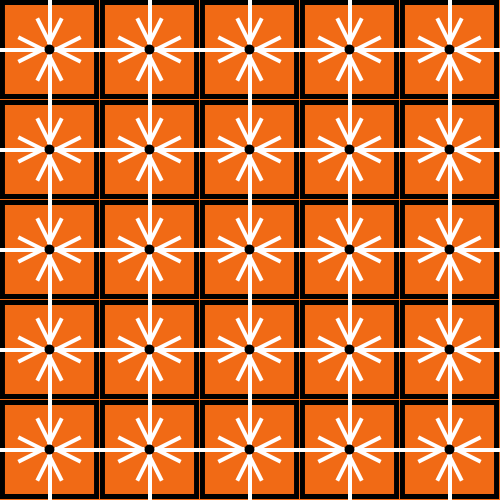
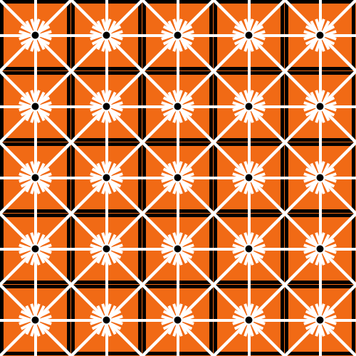
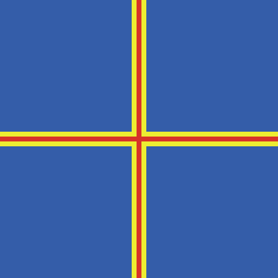
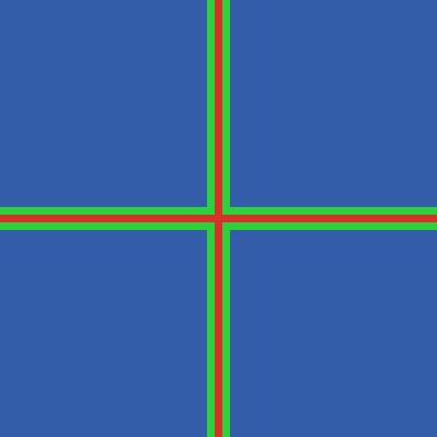
(a) Von Neumann neighborhoods on a torus

Figure 1. The figure shows the regular networks that correspond to a grid with periodic boundaries using (a) Von Neumann neighborhoods and (b) Moore neighborhoods. There is a white link between any two patches that are neighbors.

A network is a set of nodes and a set of links. Nodes represent the agents and links connect agents that are neighbors. Figure 1 shows, in white, the links corresponding to a 2-dimensional grid with toroidal topology, using Von Neumann neighborhoods (fig. 1(a)) and using Moore neighborhoods (fig. 1(b)).

Here we consider regular undirected networks only. Undirected networks are those where the neighborhood relationship is symmetric, i.e., if agent a is a neighbor of agent b, then agent b is also a neighbor of agent a. Regular networks are networks where every node has the same degree (i.e., the same number of neighbors). Thus, the spatial grids we have considered in this chapter, with periodic boundaries, fit the definition of regular undirected networks.^[9]

For simplicity, here we consider games with two strategies only. Let us denote them $A$ and $B$ . Our goal is to derive a system of differential equations for the (joint) evolution of:

the fraction of agents using strategy $A$ , and
the conditional probability that a neighbor of an $A$ -player is an $A$ -player.

The following section explains the notation we will use.

3.2.1. Notation

Notation for nodes (i.e., agents)

$N$ is the number of agents.
$k$ is the number of neighbors (or degree) of every agent.
$[A]$ is the number of agents with strategy $A$ , and $[B]$ is the number of agents with strategy $B$ . Thus, $[B] = N - [A]$ .
$x_A = \frac{[A]}{N}$ is the fraction of players using strategy $A$ . Similarly, $x_B = \frac{[B]}{N}$ . Therefore, $x_B = 1 - x_A$ .

Notation for links

We follow the convention of counting links between agents as if they were directed, i.e., if an $A$ -player and a $B$ -player are neighbors, we count two links: one $A$ – $B$ link and one $B$ – $A$ link.^[10] Thus, the total number of links is $k N$ .

$[AB]$ denotes the number of links from $A$ -players to $B$ -players. We define $[AA]$ , $[BA]$ and $[BB]$ analogously. Thus, we have $[AA] + [AB] + [BA] + [BB] = kN$ and $[BA] = [AB].$
$x_{AB} = \frac{[AB]}{k N}$ denotes the fraction of links from $A$ -players to $B$ -players. We define $x_{AA}$ , $x_{BA}$ and $x_{BB}$ analogously. Thus, we have $x_{AA} + x_{AB} + x_{BA} +x_{BB} = 1$ and $x_{AB} = x_{BA}$ .
$q_{A/A} = \frac{[AA]}{[AA] + [AB]} = \frac{[AA]}{k [A]} = \frac{x_{AA}}{x_A}$ denotes the fraction of neighbors of $A$ -players that are $A$ -players themselves. This is also the probability that a (random) neighbor of a (random) $A$ -player is an $A$ -player. $q_{B/A} = \frac{[AB]}{[AA] + [AB]} = \frac{x_{AB}}{x_A} = 1 - q_{A/A}$ is the probability that a random neighbor of an $A$ -player is a $B$ -player. We have equivalent definitions for $q_{A/B} = \frac{x_{AB}}{x_B}= \frac{x_{A}}{1-x_A} (1-q_{A/A})$ and for $q_{B/B} = 1-q_{A/B}$ .

Importantly, note that all the considered variables $x_{X}$ , $x_{XY}$ and $q_{X/Y}$ can be expressed as functions of $x_A$ and $q_{A/A}$ .

3.2.2. Neighborhood configurations

In this section we derive the probability of different neighborhood configurations. We assume that the model is such that the only relevant information about the neighborhood is its distribution of strategies. With two strategies, this distribution can be characterized by the number of $A$ -neighbors, $k_A$ , with $0 \leq k_A \leq k$ .

For an $A$ -player, the probability of being in a neighborhood with $k_A$ $A$ -neighbors can be approximated by the following binomial distribution:

$P_A(k_A) = {k \choose k_A} q_{A/A}^{k_A} (1 - q_{A/A})^{k - k_A}$

And, for a $B$ -player, the probability of being in a neighborhood with $k_A$ $A$ -neighbors can be approximated by:

$P_B(k_A) = {k \choose k_A} q_{A/B}^{k_A} (1 - q_{A/B})^{k - k_A}$

It will also be useful to refine these probabilities for the cases where we already know that there is a player in the neighborhood using a strategy different from the focal agent’s strategy. That is, if we already know that (at least) one of the neighbors of a focal $A$ -player is a $B$ -player, the conditional probability of the neighborhood configuration with $k_A$ $A$ -players for the focal $A$ -player can be approximated, for $k_A \leq k-1$ , by

$P_{A,\text{One}B}(k_A) = {{k-1} \choose k_A} q_{A/A}^{k_A} (1 - q_{A/A})^{k-1 - k_A}$

And, equivalently, for a $B$ -player with at least one $A$ -neighbor, the conditional probabilities, for $k_A \geq 1$ , are given by

$P_{B,\text{One}A}(k_A) = {{k-1} \choose {k_A-1}} q_{A/B}^{k_A-1} (1 - q_{A/B})^{k - k_A}$

Importantly, note that, given that $q_{A/B} = \frac{x_{A}}{1-x_A} (1-q_{A/A})$ , all the formulas in this subsection can also be expressed in terms of $x_A$ and $q_{A/A}$ .

3.2.3. Derivation of the first equation: $\dot{x}_A = f_1(x_A, q_{A/A})$

As indicated before, our goal is to derive a system of differential equations for i) the fraction of agents using strategy $A$ and ii) the conditional probability that a neighbor of an $A$ -player is an $A$ -player, i.e.,

$\begin{align*} \dot{x}_A &= f_1(x_A, q_{A/A}) \\ \dot{q}_{A/A} &= f_2(x_A, q_{A/A}) \end{align*}$

To derive the first equation, we follow the same approach we used to derive the mean dynamic (section 1.4.3.2.1). We define one unit of clock time as the time over which every agent is expected to receive exactly one revision opportunity. Thus, over the time interval $dt$ , the number of agents who are expected to receive a revision opportunity is $N dt$ . Let $\mathbb{P}(A \rightarrow B)$ be the probability that a revising $A$ -player switches to strategy $B$ . Therefore, of the $N dt$ agents who revise their strategies, $x_A \,\mathbb{P}(A \rightarrow B) N dt$ are expected to switch from strategy $A$ to strategy $B$ . Similarly, $x_B \,\mathbb{P}(B \rightarrow A) N dt$ agents are expected to switch from strategy $B$ to strategy $A$ . Hence, the expected change in the number of agents that are using strategy $A$ over the time interval $dt$ is $(x_B\, \mathbb{P}(B \rightarrow A)- x_A\,\mathbb{P}(A \rightarrow B))N dt$ . Therefore, the expected change in the fraction of agents using strategy $A$ is:

$dx_A = \frac{1}{N}\left(x_B\,\mathbb{P}(B \rightarrow A) - x_A\,\mathbb{P}(A \rightarrow B)\right)N dt = \left(x_B\,\mathbb{P}(B \rightarrow A) - x_A\,\mathbb{P}(A \rightarrow B)\right) dt$

Thus,

$\dot{x}_A = x_B\,\mathbb{P}(B \rightarrow A)-x_A\,\mathbb{P}(A \rightarrow B)$

Note, however, that the probabilities in the formula above depend on the neighborhood configuration of the focal agent. Thus, we should consider all the possible neighborhood configurations and their corresponding probabilities, as follows:

$\dot{x}_A = x_B \sum_{k_A = 0}^k P_B(k_A) F_B(k_A) - x_A \sum_{k_A = 0}^k P_A(k_A) F_A(k_A)$

where $F_B(k_A)$ is the (conditional) probability that a revising $B$ -player with $k_A$ $A$ -neighbors switches to strategy $A$ , and $F_A(k_A)$ is the (conditional) probability that a revising $A$ -player with $k_A$ $A$ -neighbors switches to strategy $B$ .

Conditional switching probabilities $F_B(k_A)$ and $F_A(k_A)$

Conditional switching probabilities depend on the number of $A$ -neighbors $k_A$ and on the decision rule. As decision rule, here we focus on the imitative-pairwise-difference rule; we leave the derivation of the switching probabilities for other decision rules as exercises at the end of this section.

Under the imitative-pairwise-difference rule, the revising agent looks at a random neighbor and, if the observed neighbor has a greater average payoff, the reviser copies her strategy with probability proportional to the difference in average payoffs. Thus, let us start defining the payoff functions.

Consider first a revising $B$ -player with $k_A$ $A$ -neighbors. The average payoff to such a revising $B$ -player is $\pi_B(k_A) = (k_A \pi_{BA} + (k-k_A) \pi_{BB})/k$ .^[11] The payoff to an $A$ -neighbor of the revising $B$ -player depends on the number $k'_A \leq k-1$ of $A$ -neighbors of this $A$ -player (who has at least one $B$ -neighbor), and this payoff is $\pi_A(k'_A)= (k'_A \pi_{AA} + (k-k'_A) \pi_{AB})/k$ .

We can now derive $F_B(k_A)$ , which is the probability that a revising $B$ -player switches to strategy $A$ . The probability that a random neighbor of a revising $B$ -player with $k_A$ $A$ -neighbors is an $A$ -player is $\frac{k_A}{k}$ . The payoff of this random $A$ -neighbor depends on the number $k'_A$ of $A$ -neighbors she has, with $0 \le k'_A \le k-1$ (since we know that she has at least one $B$ -neighbor, i.e. the reviser). The probability that the observed $A$ -neighbor has $k'_A$ $A$ -neighbors is $P_{A,\text{One}B}(k'_A)$ . Therefore, the formula for $F_B(k_A)$ reads:

$F_B(k_A) = \frac{k_A}{k} \sum_{k'_A=0}^{k-1} P_{A,\text{One}B}(k'_A) \frac{[\pi_A(k'_A)-\pi_B(k_A) ]^+}{\Delta},$

where $[x]^+ = \max(x,0)$ and $\Delta>0$ is a sufficiently large constant to guarantee that $\frac{[\pi_A(k'_A)-\pi_B(k_A) ]^+}{\Delta} \le 1$ in every possible case.^[12]

Following the same reasoning, we can derive $F_A(k_A)$ :

$F_A(k_A) = \frac{k-k_A}{k} \sum_{k'_A=1}^k P_{B,\text{One}A}(k'_A) \frac{[\pi_B(k'_A)-\pi_A(k_A) ]^+}{\Delta}$

Substitution

By now, we have the formulas for every term in the equation:

$\dot{x}_A = x_B \sum_{k_A = 0}^k P_B(k_A) F_B(k_A) - x_A \sum_{k_A = 0}^k P_A(k_A) F_A(k_A)$

It only remains to express all these terms as functions of $x_A$ and $q_{A/A}$ to obtain the first equation of the pair approximation:

$\dot{x}_A = f_1(x_A, q_{A/A})$

3.2.4. Derivation of the second equation: $\dot{q}_{A/A} = f_2(x_A, q_{A/A})$

Recall that $q_{A/A} = \frac{x_{AA}}{x_A}$ . Therefore,

$\dot{q}_{A/A} = \frac{\dot{x}_{AA}}{x_A} - \frac{x_{AA}}{x_A^2} \dot{x}_A$

Since we already have the formula for $\dot{x}_A = f_1(x_A, q_{A/A})$ , we just need to derive $\dot{x}_{AA}$ .

Remember that $x_{AA} = \frac{[AA]}{k N}$ . Just like we did for the first equation, here we also consider the events that modify $[AA]$ , taking into account all the possible neighborhood configurations with their corresponding probabilities. The expected change in the number of $A$ – $A$ links $[AA]$ over the time interval $dt$ is:

$d[AA] = \left(x_B \sum_{k_A = 0}^k P_B(k_A) F_B(k_A) L^+_B(k_A) - x_A \sum_{k_A = 0}^k P_A(k_A) F_A(k_A) L^-_A(k_A) \right) Ndt,$

where $L^+_B(k_A) = 2 k_A$ is the number of new $A$ – $A$ links that appear when a $B$ -player with $k_A$ $A$ -neighbors switches to strategy $A$ , and where $L^-_A(k_A) = 2 k_A$ is the number of $A$ – $A$ links that disappear when an $A$ -player (with $k_A$ $A$ -neighbors) adopts strategy $B$ . Therefore, the expected change in $x_{AA}$ is:

$dx_{AA} = \frac{d[AA]}{k N} = \frac{1}{k} \left(x_B \sum_{k_A = 0}^k P_B(k_A) F_B(k_A) L^+_B(k_A) - x_A \sum_{k_A = 0}^k P_A(k_A) F_A(k_A) L^-_A(k_A) \right) dt$

Thus,

$\dot{x}_{AA} = \frac{1}{k} \left(x_B \sum_{k_A = 0}^k P_B(k_A) F_B(k_A) L^+_B(k_A) - x_A \sum_{k_A = 0}^k P_A(k_A) F_A(k_A) L^-_A(k_A) \right)$

Expressing the different terms as functions of $x_A$ and $q_{A/A}$ , we obtain an equation of the form $\dot{x}_{AA} = f_3(x_A, q_{A/A})$ . Finally, from $\dot{q}_{A/A} = \frac{\dot{x}_{AA}}{x_A} - \frac{x_{AA}}{x_A^2} \dot{x}_A$ , we obtain the second equation of the pair approximation $\dot{q}_{A/A} = f_2(x_A, q_{A/A})$ .

3.3. Solving the pair approximation. Examples

Just like we did with the mean dynamics, we can numerically solve the system of differential equations of the pair approximation. To this end, we have created a Mathematica^® notebook that you can download and run using the free Wolfram Player. Figure 2 shows its interface.

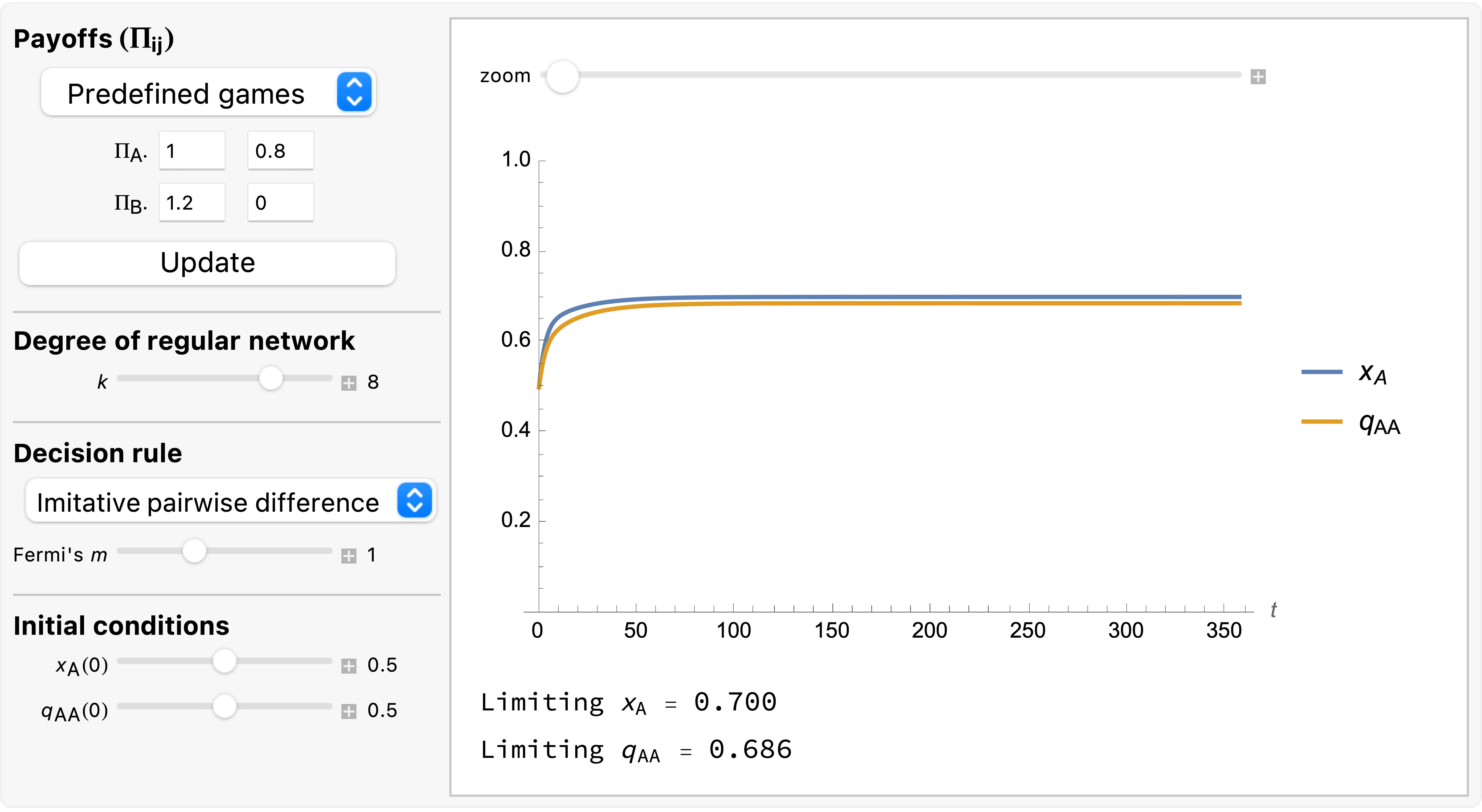
Figure 2. Interface of the *Mathematica*^® notebook created to solve the system of differential equations of the pair approximation (Izquierdo et al., 2024). You can download the notebook at https://github.com/luis-r-izquierdo/pair-approximation.

As an example of a case where the pair approximation works well, we present some results for the snowdrift game (payoffs = [[1 0.8][1.2 0]]) played synchronously on a 100×100 torus using Moore neighborhoods ( $k=8$ ) and the imitative-pairwise-difference rule. Initial conditions are random, with half the population using strategy $A$ and the other half using strategy $B$ , so $x_A(0) = 0.5$ and $q_{A/A}(0) \approx 0.5$ . Figure 3 shows the solution trajectory of the pair approximation (see also Figure 2), together with the average, minimum and maximum values of the fraction of $A$ -strategists at every tick, across 1000 simulation runs conducted with our nxn-imitate-best-nbr-extended model.

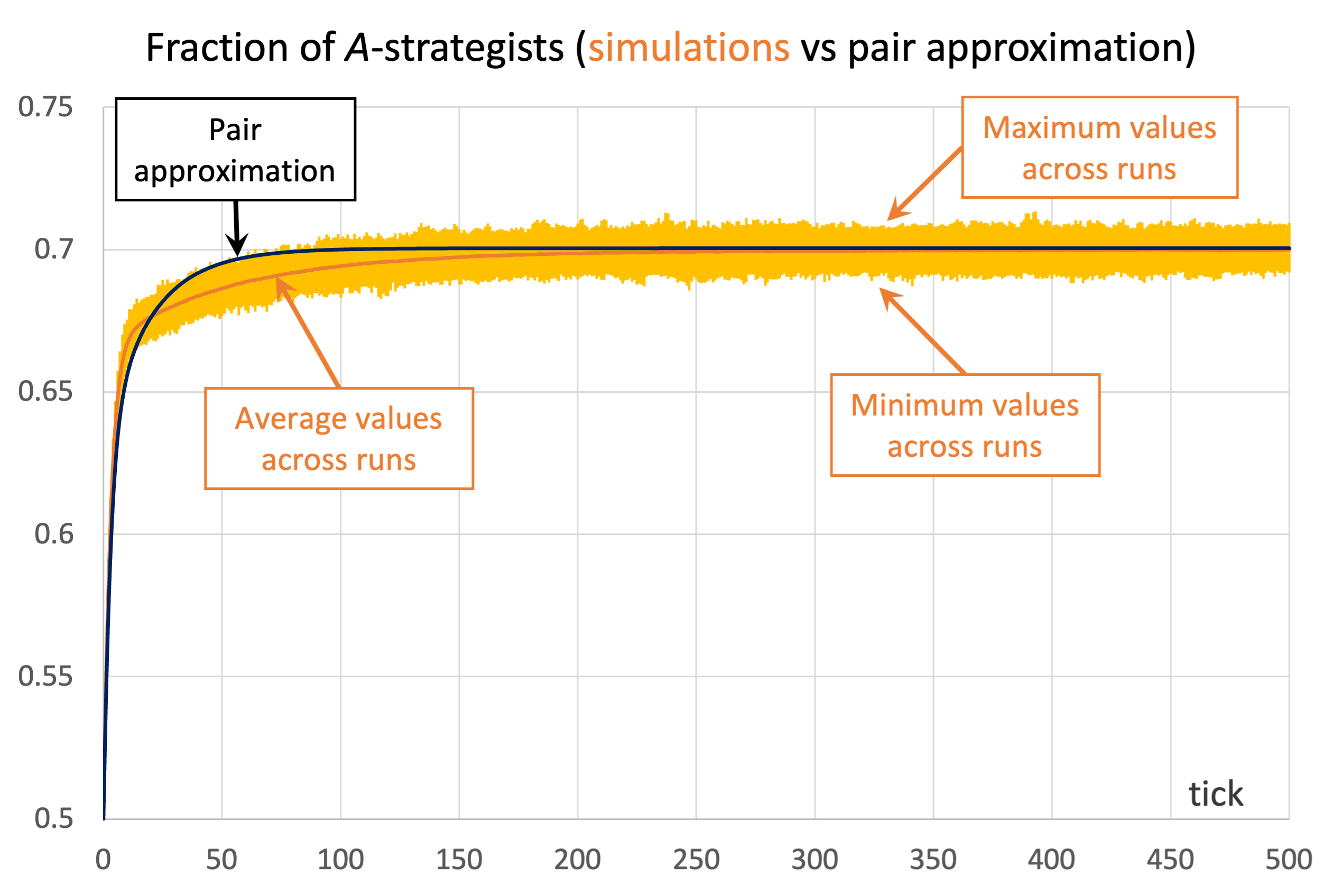Figure 3. Pair approximation and simulation results for the snowdrift game played synchronously on a 100×100 torus using Moore neighborhoods ( $k=8$ ) and the imitative-pairwise-difference rule. The black solid line shows the fraction of $A$ -strategists according to the pair approximation, while the orange solid line shows the average values across 1000 simulation runs. The orange error bars show the minimum and maximum values observed across the 1000 runs. Payoffs [[1 0.8][1.2 0]]; initial conditions [5000 5000].

As you can see in Figure 3, in this case the pair approximation works reasonably well, and its limiting value $x_A^{\infty} \equiv \lim_{t \rightarrow \infty} x_A(t) = 0.70$ provides a very good estimate of the long-term average value of the fraction of $A$ -strategists.^[13]

Unfortunately, the pair approximation does not always work so well, by any means. As an example, Figure 4 shows results for the same parameterization as in Figure 3, but using Von Neumann neighborhoods ( $k=4$ ) instead of Moore neighborhoods.

Figure 4. Pair approximation and simulation results for the snowdrift game played synchronously on a 100×100 torus using Von Neumann neighborhoods ( $k=4$ ) and the imitative-pairwise-difference rule. The black solid line shows the fraction of $A$ -strategists according to the pair approximation, while the orange solid line shows the average values across 100 simulation runs. The orange error bars show the minimum and maximum values observed across the 100 runs. Payoffs [[1 0.8][1.2 0]]; initial conditions [5000 5000].

In the case shown in Figure 4, the pair approximation provides an estimate for the long-term average fraction of $A$ -strategists of $x_A^{\infty} = 0.67$ , which is far from the value of 0.94 obtained by running the stochastic model.^[14]

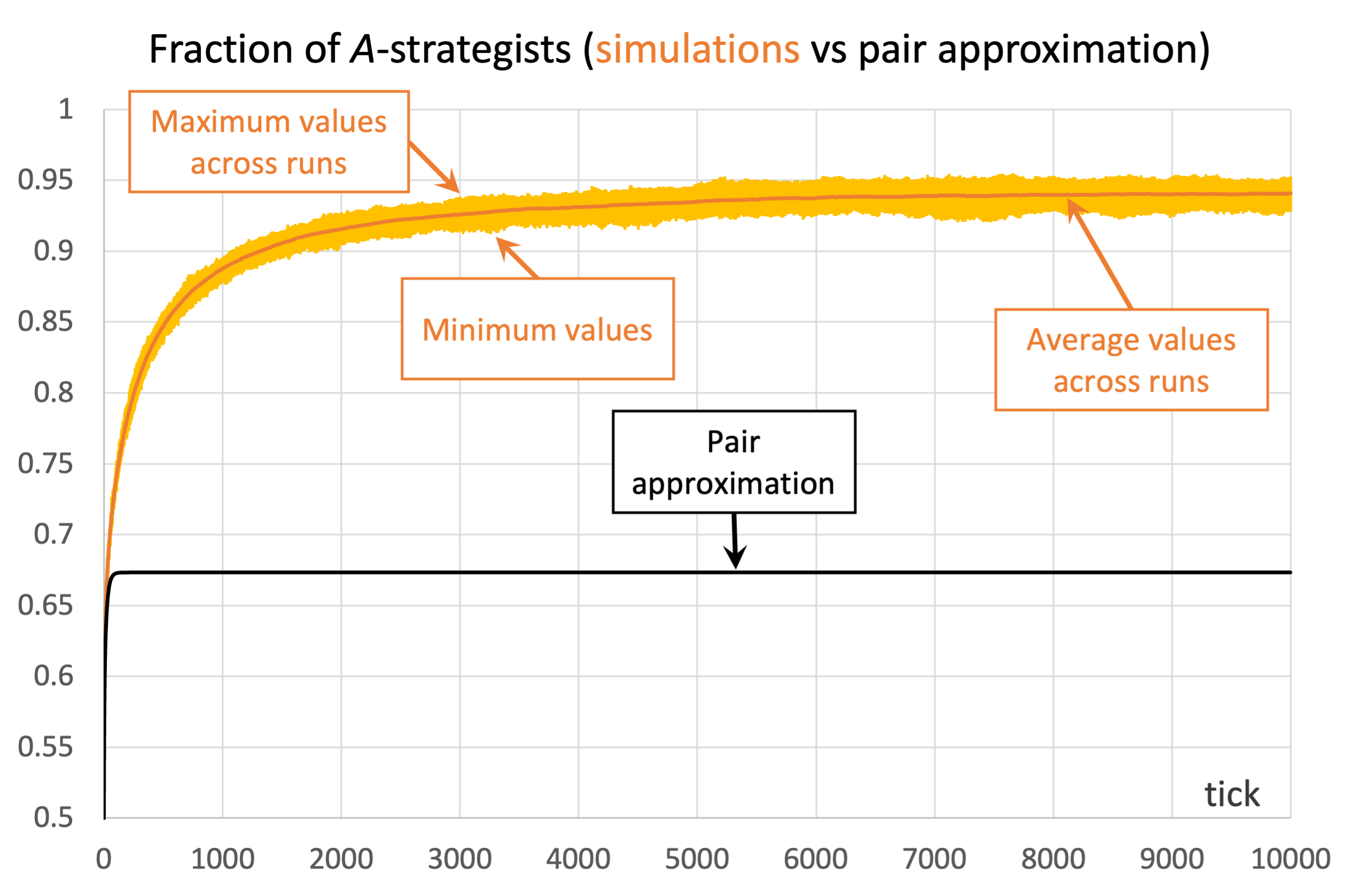
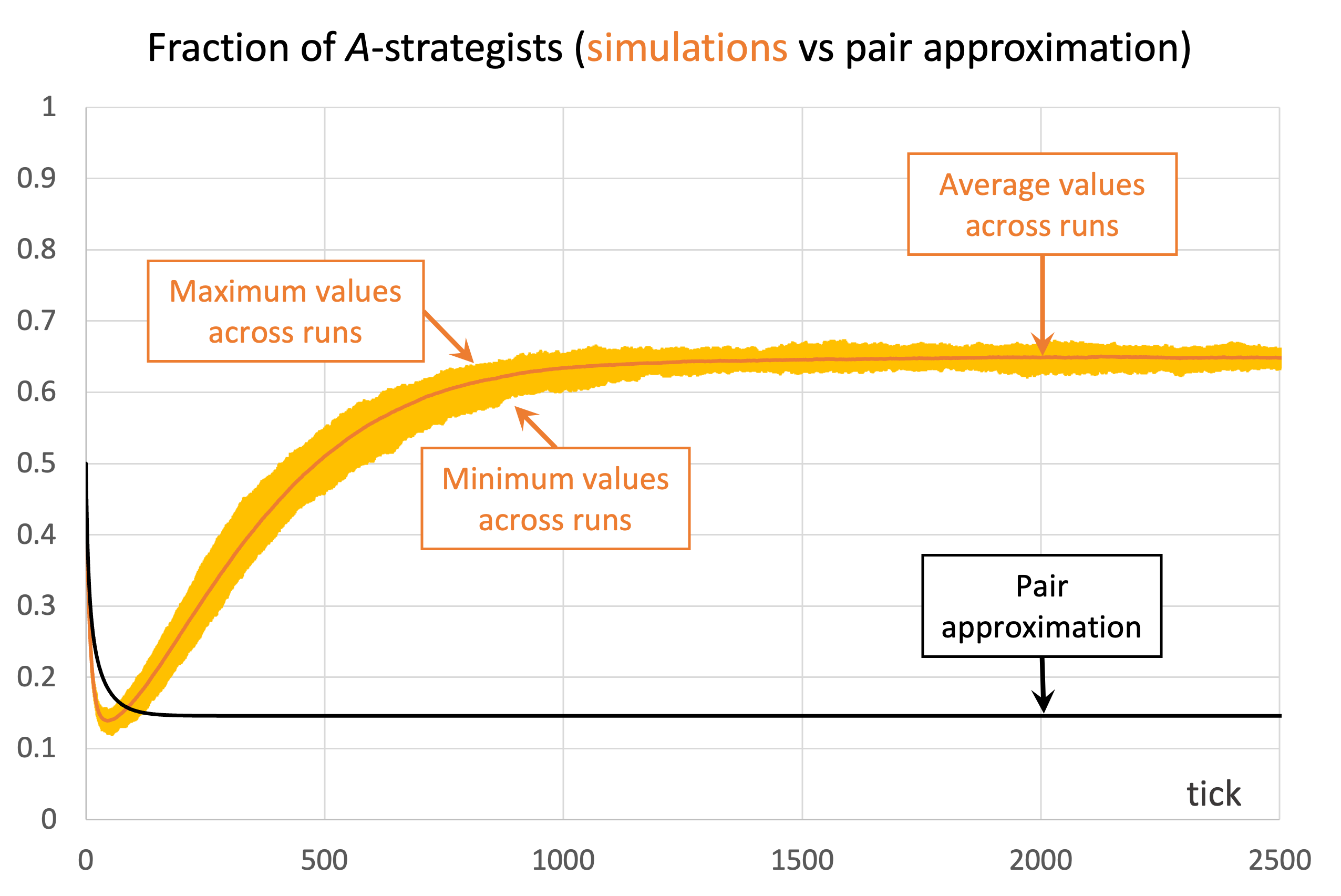
We conclude this section with another example where the pair approximation does not work well. Consider the Prisoner’s Dilemma with payoffs [[1 0][1.1 0.1]] played asynchronously on a 125×125 torus using Moore neighborhoods ( $k=8$ ) and the imitative-pairwise-difference rule. Initial conditions are such that $x_A(0) \approx q_{A/A}(0) \approx 0.5$ . Figure 5 shows the comparison between the pair approximation and a computational experiment run with our nxn-imitate-best-nbr-extended model.^[15] In this case, the pair approximation provides an estimate for the long-term average fraction of $A$ -strategists of $x_A^{\infty} = 0.15$ , while the value obtained from the computational experiment is 0.65.

Figure 5. Pair approximation and simulation results for the Prisoner’s Dilemma played asynchronously on a 125×125 torus using Moore neighborhoods ( $k=8$ ) and the imitative-pairwise-difference rule. The black solid line shows the fraction of $A$ -strategists according to the pair approximation, while the orange solid line shows the average values across 100 simulation runs. The orange error bars show the minimum and maximum values observed across the 100 runs. Payoffs [[1 0][1.1 0.1]]; initial conditions [[7812 7813].

The take-home message of these examples is that the pair approximation may or may not work well, and in most cases there is no simpler or shorter way of finding out whether it will work well other than running the computer simulations.

3.4. Discussion

Note that in the “well-mixed population” models we developed in chapter 1, every player was equally likely to interact with every other player, regardless of their strategies. Thus, in those models $q_{A|A} = q_{A|B} = x_A$ .

By contrast, in spatial models, the values of $x_A$ and $q_{A|A}$ generally differ, and we often obtain better approximations if we track their joint evolution, as we do in the pair approximation. However, it seems clear that in most cases these two variables will not be enough to condense all the relevant information that can affect evolutionary dynamics on grids (or, more generally, on networks). To make this important point crystal clear, below we present different network configurations with exactly the same initial values of $x_A$ and $q_{A|A}$ (so the prediction of the pair approximation is exactly the same for both), but with completely different evolution.

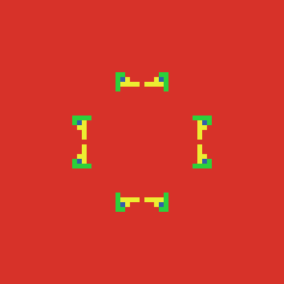
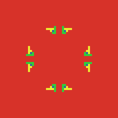
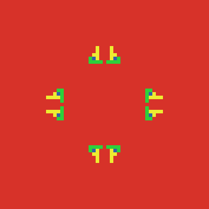
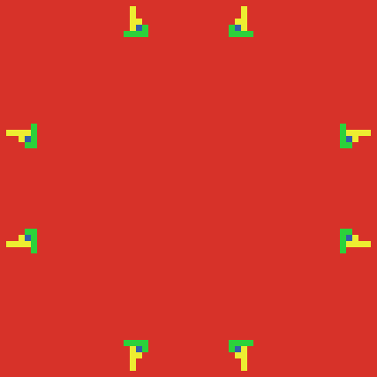
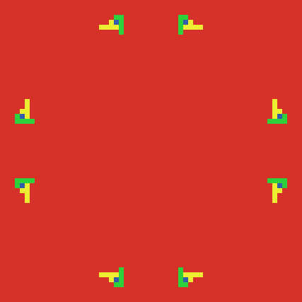
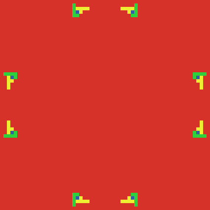
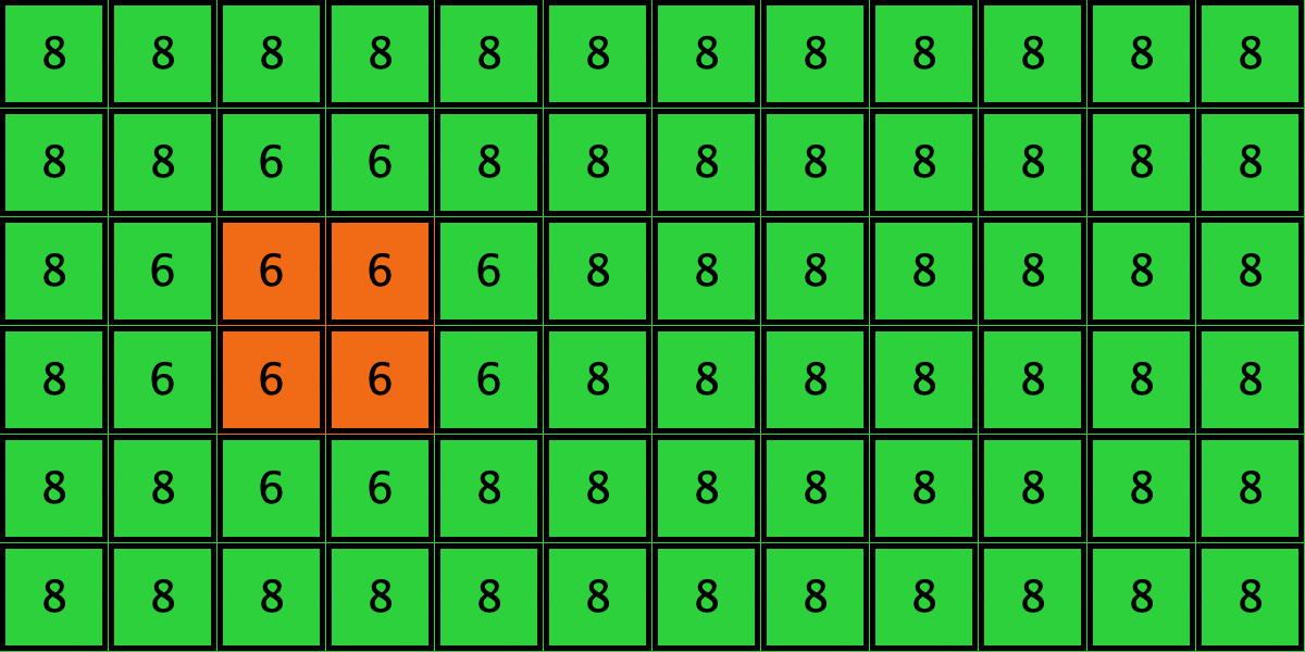
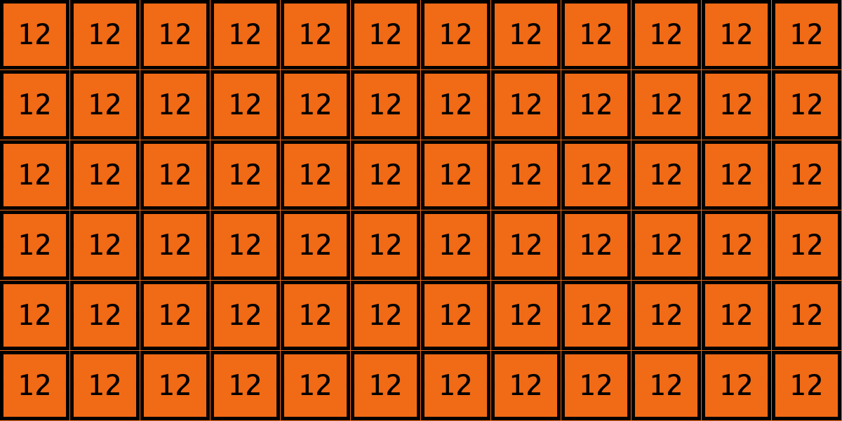
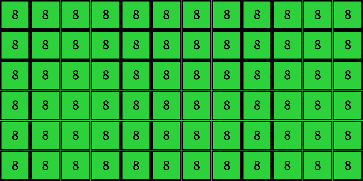
Consider a toroidal grid with Von Neumann neighborhoods ( $k=4$ ). Agents play a coordination game with strategies $A$ (orange) and $B$ (green), and payoff matrix [[3 0][0 2]], using the imitate-if-better-all-nbrs decision rule. You may assume synchronous or asynchronous updating. Initially, all players are using the green strategy $B$ except for a group of 8 agents who use strategy $A$ . See the two initial configurations in Table 3 below for two examples. These initial configurations show only the part of the grid corresponding to the 8 orange $A$ -strategists and their second neighbors; the numbers are the total payoff obtained by each player. You may assume that the grid is larger than the part shown in the figures, as long as the part not shown is green.

Table 3 shows two distinct initial configurations, each with 8 $A$ -strategists and 8 undirected $A$ – $A$ links, so they both have the same values for $x_A$ and $q_{A|A}$ . However, configuration c1 is an absorbing state (i.e., it does not change over time), while configuration c2 leads to a complete invasion by orange strategy $A$ .

Name	Initial configuration	====>	Final configuration
c1		====>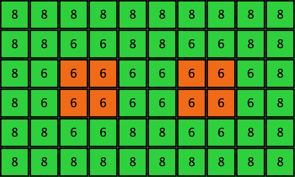
c2		====>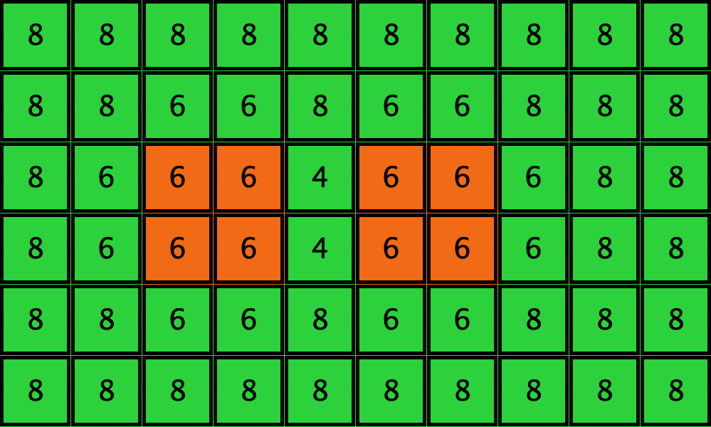

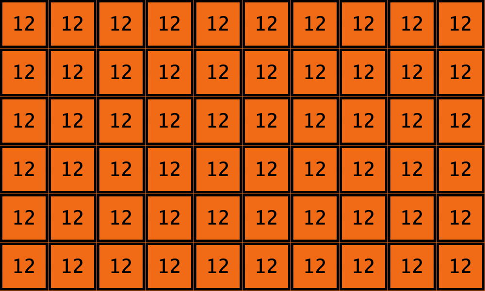Table 3. Two initial configurations with the same values for $x_A$ and $q_{A|A}$ , and their corresponding final states.

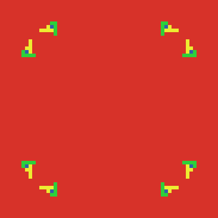
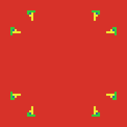
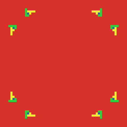
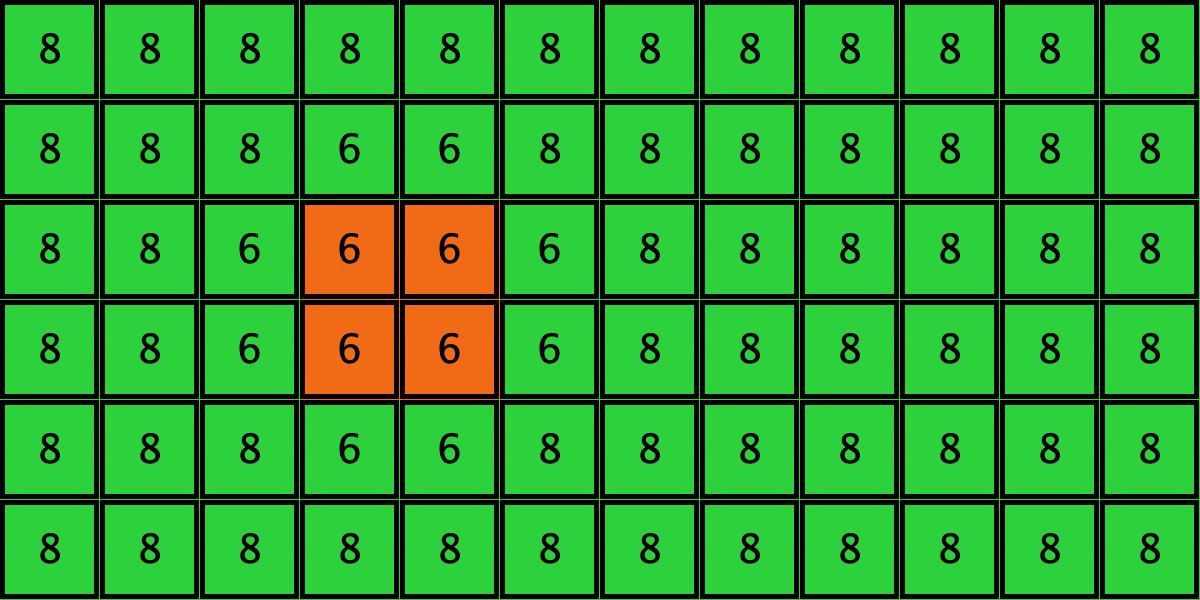
Similarly, initial configurations c3 to c6 in Table 4 share the same number of $A$ -strategists (8) and of $A$ – $A$ links (7 undirected links), so they all present the same values for $x_A$ and $q_{A|A}$ . However, their dynamic evolution is completely different:

Configuration c3 leads to the survival of the 2×2 orange square block and the disappearance of the other orange $A$ -players.
Configuration c4 leads to a complete invasion by orange strategy $A$ .
Configuration c5 leads to a complete invasion by green strategy $B$ .
Configuration c6 may lead to the invasion of orange $A$ , to the invasion of green $B$ , or to one of two other possible final states where both strategies are present.

Name	Initial configuration	====>	Possible final configurations
c3		====>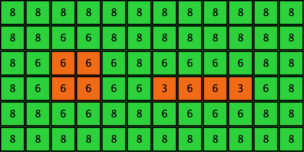
c4		====>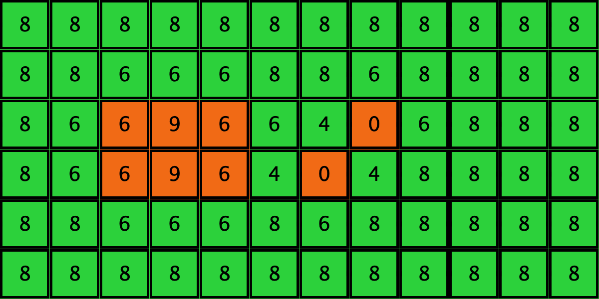
c5		====>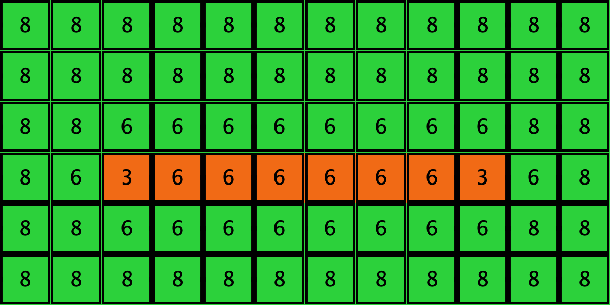
c6		====>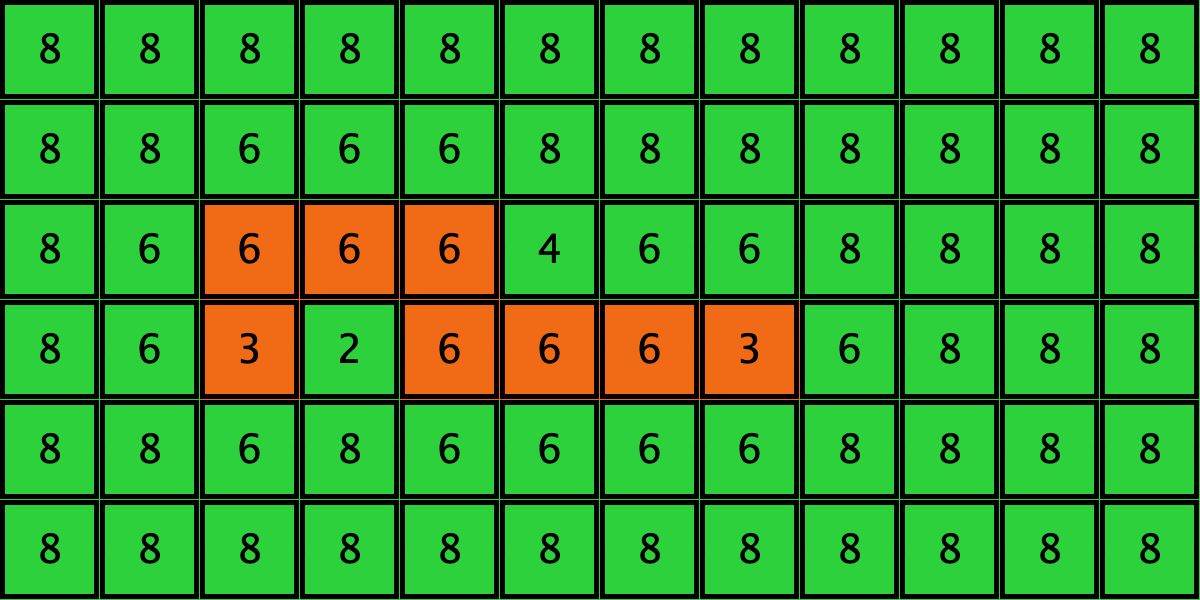

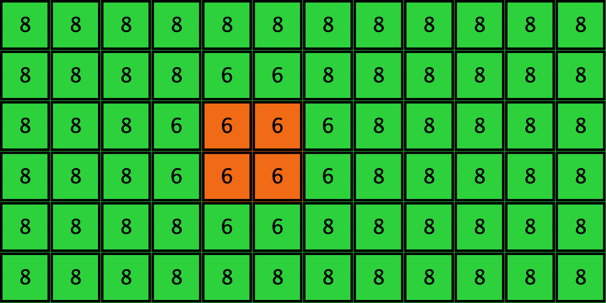Table 4. Four initial configurations with the same values for $x_A$ and $q_{A|A}$ , and the final states they may lead to.

It is then clear that variables $x_A$ and $q_{A|A}$ are not sufficient to condense all the relevant information that can affect evolutionary dynamics on grids.^[16] Thus, in general, the pair approximation presented here cannot provide a good description of the agent-based stochastic dynamics.

One may wonder whether adding more variables may lead to better approximations. There are different ways we can generalize and improve the pair approximation we have derived here. For instance, if the underlying network is such that neighboring nodes tend to have common neighbors (i.e., high clustering coefficient), we may refine the estimation of the probability of a neighbor’s neighborhood configuration (i.e., our terms $P_{A,\text{One}B}(k'_A)$ and $P_{B,\text{One}A}(k'_A)$ ) by taking into account these correlations (see, e.g., Morita (2008)). Similarly, to estimate the probability $q_{X|AB}$ that a (random) neighbor of an $A$ -player linked to a $B$ -neighbor is an $X$ -player (with $X\in \{A,B\}$ ), we could keep track of the expected evolution of triplets, such as [AAB]. This could well improve the quality of the approximation, but it would also increase the number of variables and equations in the system of ODEs, possibly making it less amenable to analysis (van Baalen, 2000).

In any case, the bottom line is that there is no guarantee whatsoever that adding more variables will eventually yield a good analytical approximation that will work in every case. While for unstructured populations there are mathematical theorems that guarantee that the stochastic process converges to the mean dynamic as the population size grows, this is not generally the case for pair approximations in structured populations. The “validity” of pair approximations is generally assessed via simulations… the very same simulations the approximation aims to describe.

We conclude with a quote by Fu et al. (2010) which nicely summarizes the role of the pair approximation in understanding evolutionary dynamics on grids:

[The pair approximation] provides important qualitative insights into the invasion dynamics but often fails to provide accurate quantitative predictions. Fu et al. (2010, p. 360)

4. Exercises

Exercise 1. Derive the pair approximation for the imitate-if-better-all-nbrs decision rule.

Exercise 2. Derive the pair approximation for the Fermi-m decision rule.

Exercise 3. Derive the pair approximation for the imitate the best neighbor decision rule. For simplicity, you may want to assume that a revising $B$ -player will change her strategy only if no $B$ -player achieves the maximum payoff in the neighborhood (and analogously for $A$ -revisers). This is a slightly different way of resolving ties. Warning! This exercise is significantly harder than the two previous ones.

^CODEExercise 4. Extend our nxn-imitate-best-nbr-extended model to include two monitors that show the values of $x_A$ and $q_{A|A}$ .

Exercise 5. In exercise 2.3.1, we parameterized our nxn-imitate-best-nbr-extended model to replicate the simulation results shown in figures 1b and 1d of Hauert and Doebeli (2004). We can now replicate their pair approximation results too (i.e., the solid line in these figures). Please, use the Mathematica notebook that solves the pair approximation to compute a few values of the solid lines in these two figures.

Exercise 6. How can we parameterize our nxn-imitate-best-nbr-extended model and the Mathematica notebook that solves the pair approximation to replicate the results shown in figures 4a, 4d, 6a and 6c of Fu et al. (2010)?

You can run your own simulations of the Game of Life using the following Mathematica script:

globalState = RandomInteger[1, {50, 50}];
Dynamic[ArrayPlot[
  globalState = Last[CellularAutomaton["GameOfLife", globalState, 1]]
]]

↵

Two useful references to learn about the fascinating world of cellular automata are Berto and Tagliabue (2023) and Wolfram (2002). Sigmund (1983, chapter 2) and Mitchell (1998) are two wonderful thought-provoking gems, highly recommended for anyone interested in appreciating the important role of cellular automata in understanding self-reproduction and universal computation. ↵
Note, however, that the neighborhood in the definition of the corresponding cellular automaton is not the (Moore) neighborhood used in the model. In the model, the strategy of a player depends on the payoffs of its Moore neighbors, which in turn depend on the strategy of the player's neighbors' neighbors. Thus, the neighborhood of the corresponding cellular automaton is the Moore neighborhood of range 2, i.e., the 5x5 square around each patch. ↵
Szabó and Fáth (2007, sections 4.1 and 6.5) discuss this model in detail and review several other CA models in the context of evolutionary game theory. ↵
Wolfram (2002, p. 739) calls this feature "computational irreducibility". However, to our knowledge, there is not a unique and uncontested formal definition of this concept. ↵
This is a slightly extended version of table 1 in Nowak and May (1993, p. 46). ↵
We use the term "fixed boundaries" to be consistent with Nowak and May's (1992, 1993) original papers, but other authors, such as Sayama (2015, p. 189), refer to this topology as "cut-off boundaries", and use the term "fixed boundaries" for a different topology. ↵
In section 1.4.3.1.3 we provided sufficient conditions for irreducibility and aperiodicity of time-homogeneous Markov chains. ↵
Hauert and Szabó (2005, section B) study dynamics on different regular undirected networks besides lattices, such as random regular graphs and regular small world networks. ↵
This convention is convenient for the formulas, but there are alternatives that are also valid. ↵
For decision rules that depend on total payoffs, rather than on average payoffs, we would just multiply by $k$ . ↵
The value of $\Delta$ should be at least $\left(\max(\pi_{AA},\pi_{AB},\pi_{BA},\pi_{BB}) - \min(\pi_{AA},\pi_{AB},\pi_{BA},\pi_{BB})\right)$ ; choosing any value greater than this will only imply a change of speed in the differential equations. ↵
For asynchronous updating, the match between the pair approximation and the simulations is slightly worse but qualitatively similar. The long-term average values for synchronous and asynchronous updating, together with the pair approximation, are plotted in figure 1d of Hauert and Doebeli (2004), entering a cost-to-benefit ratio of 0.2. ↵
These values are plotted in figure 1b of Hauert and Doebeli (2004), entering a cost-to-benefit ratio of 0.2. ↵
A similar figure can be found in Fu et al. (2010, figure 4a, red lines), though they use different initial conditions. The limiting values ( $x_A^{\infty} = 0.15$ and the value obtained from the computational experiment, 0.65) are also plotted in figure 6a of Fu et al. (2010), for $u=0.1$ . Fu et al. (2010) use total payoffs rather than average payoffs, but this difference is irrelevant when using the imitative-pairwise-difference rule on regular networks. ↵
Hauert and Szabó (2005, figure 5) show examples of different regular networks that share the same pair approximation but have very different dynamics. ↵

License

Icon for the Creative Commons Attribution 4.0 International License

Agent-Based Evolutionary Game Dynamics (IN PROGRESS) Copyright © 2024 by Luis R. Izquierdo, Segismundo S. Izquierdo & William H. Sandholm is licensed under a Creative Commons Attribution 4.0 International License, except where otherwise noted.