
Biocore Statistics Primer
Chapter 7: A Brief Introduction to Some Additional Topics
Section 7.1: Sample Size Determination
A key component of experimental design is sample size determination. How do scientists choose sample sizes that will yield sufficient, high quality data that they can confidently use to test hypotheses and address research questions?
Here we provide some guidance for the selection of sample sizes. A mathematically complete description of this is beyond the scope of this Primer. However, the ideas presented will provide useful initial guidelines for designing studies in practice.
We focus on the two independent-sample situation since this is what is used most frequently for sample size calculations. Previously (in chapter 3 and chapter 4), we indicated that there were two types of error we could make. The sample data we collect can lead us to reject a null hypothesis when the null really is true, and can also cause us to fail to reject the null if it is really false. (These are denoted as Type I and Type II errors respectively.) However, when the null is false, there are many ways that it could be false. For the thistle example from the previous chapter, Ho : [latex]\mu_1 = \mu_2[/latex] and HA : [latex]\mu_1 \neq \mu_2[/latex]. The null will be false if [latex]\mu_1- \mu_2 =[/latex] 20, or 5, or 1 or even 0.1 (and similarly if these values are negative).
In practical situations, researchers designing studies use their scientific understanding to select a “difference of interest” that they would like to detect. (Scientists often choose a difference of interest from a careful review of literature and/or their own prior observations). For example, suppose that prairie ecologists decide that a difference of 3 thistles per quadrat, between the burned and unburned treatments, is scientifically meaningful and they wish to design a study capable of detecting this difference, if it truly exists.
From prior study — or in some cases from theoretical arguments — they will have some measure of the underlying within group variance. Let “DOI” be the difference of interest and [latex]\sigma^2[/latex] be the measure of variance available to the researchers.
DOI = (scientific) Difference of Interest
Then, a reasonable formula to give the desired sample size is
[latex]n = 20 \frac {\sigma^2}{(DOI)^2}[/latex] .
Here n is the required sample size for each group. (A balanced design is assumed.) This exact formula will not appear in most text books. In text books, the number 20 will be replaced by some terms that include “Z” (representing the standard normal distribution: [latex]Z\sim N(0,1)[/latex] ) which are directly related to the desired probabilities of Type I and Type II error. The value of 20 corresponds approximately to a probability of Type I error of 0.05 and a probability of Type II error of 0.11. If it is important to invoke a smaller value for either of the error probabilities, then one will need a number larger than 20; if one can tolerate larger probabilities, then one could use a number less than 20. However, in many circumstances, 20 is a usable guideline.
Let us illustrate how this might be used in practice. Suppose you wish to conduct a “thistle study” in a different prairie site. Suppose that previous studies (perhaps pilot studies) provide a plausible value for the variance of 16. Suppose the DOI — based on scientific arguments !!! — is 3.0 thistles per quadrat. A “useful” sample size can be computed as follows:
[latex]n = 20 \frac {16}{3^2} = 35.56[/latex].
We always round up. Thus, using this guideline, we would need 36 quadrats per treatment group. From the general formula, we can see that the larger the underlying variance, the larger the needed sample size will be. (This is one reason why we work hard in our experimental planning to achieve as small a variance as possible.) Similarly, the smaller the DOI, the larger the sample size will need to be.
It is important to note that practical resource constraints such as budget, equipment availability, and limited time often place limits on possible sample size. In such cases careful thought is required before proceeding with the desired study. If the limited (available) sample size leads to unacceptably high probabilities of Type I and/or Type II errors, the study will be too likely to lead to inconclusive results. In such a case, the researcher needs to rethink the study and perhaps modify the goals. Sometimes goals can be scaled back so that, with the available resources, there is a good chance of obtaining sample data that lead to conclusive scientific results. Sometimes it may be possible to add resources and, in still other situations, it may be decided that the study is not worth conducting.
Section 7.2: Simple Linear Regression
Regression analysis is among the most widely used methods in biological research. Thus, we wish to provide a brief introduction to regression analysis here.
We consider an example that could be conducted by undergraduate students. The samara is a winged seed from trees (primarily maples) that autorotates — flies like a helicopter — as it falls to the ground. The slower samaras fall, the greater the chance that the wind could disperse them over greater distances. Thus, the terminal velocity plays an important role in seed dispersal.
A useful descriptor of the aerodynamic properties of the samara is the disk loading. This is defined as [latex]W/A_d[/latex] which is the samara weight divided by the projected area of a disk swept out by the samara blade. It is known from many prior studies that the terminal velocity of samaras is proportional to the square root of the disk loading. (The units for disk loading are gm/cm2 and for terminal velocity are cm/sec.)
Terminal velocities can be measured by using photographs taken with strobe lighting as the samaras fall, with the photos taken at regular intervals. One goal of samara seed studies is to determine the relationship between disk loading and terminal velocity.
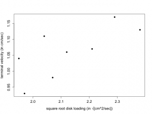
Suppose that 8 randomly selected samaras are obtained from a particular sugar maple tree (Acer saccharum) and the disk loading and terminal velocity are determined for each samara. Presented below are the square root of the disk loading (x) and the terminal velocity (y).
x:  1.97   2.12   1.95   2.38   2.21   2.04   2.29   2.07

y:  0.93   1.06   1.04   1.13   1.07   1.11   1.17   0.98
A plot of y (terminal velocity) versus x (square root of disk loading) appears in Figure 7.2.1. We note that there is a clear linear relationship although there is substantial scatter. As x increases , y also increases (linearly).
Our goal is to fit a straight line to these data. A straight line is fully described by a y-intercept and a slope. This is typically written as [latex]Y = b_0 + b_1*x[/latex] where [latex]b_0[/latex] is the y-intercept and [latex]b_1[/latex] is the slope. Figure 7.2.2 illustrates the basic idea.

In this figure the y-intercept is denoted by b (instead of [latex]b_{0}[/latex]) and the slope by m (instead of [latex]b_{1}[/latex]). The slope can be thought of as the magnitude in the increase (or decrease) in y, as x increases by one unit. It can also be viewed as the ratio of the change in y over the change in x. The y-intercept is the value of y when the regression line crosses the y-axis.
The standard method for finding the “best” straight line is to use the method of least squares. This minimizes the sum of squares of the deviations between the observed values of y and the fitted values. See Fig. 7.2.3.
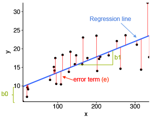
The deviations are the differences between the observed data points and the fitted line. These are denoted by the “error term” in the figure. The fitted line is determined by minimizing the sum of squares of the deviations. (This is a fairly standard mathematical procedure.)
Just like all other inferential methods, there are assumptions that underlie regression analysis. Basically, these are the same assumptions appropriate for ANOVA models described earlier. In this brief introduction, we will not provide more discussion but strongly encourage the interested reader to pursue them. They are presented in most standard statistics texts. — Here we will use R to find the “best” straight line that relates y to x for the samara seed data..
Estimates of the intercept and slope are straightforwardly obtained. The regression output is typically presented as shown in Table 7.2.1.
| estimate | st err (est) | t-value | p-value | |
| intercept | 0.276 | 0.311 | 0.887 | 0.409 |
| slope | 0.369 | 0.146 | 2.532 | 0.045 |
Thus, our estimated regression line is:
[latex]\widehat{y} = 0.276 + 0.369*x[/latex].
Here [latex]\widehat{y}[/latex] represents the fitted value.
Of most importance is the slope. As the square root of disk loading increases by 1 unit, the samara terminal velocity increases by 0.369 cm/sec. The standard error of the slope is 0.146 cm/sec. The p-value of 0.045 corresponds to the test of the null hypothesis that the slope is 0 (that is, the null hypothesis states that samara terminal velocity does not depend linearly on the square root of disk loading). Thus, at the 5% level, the p-value of 0.045 indicates that there is a significant linear relationship between samara terminal velocity and the square root of disk loading. Thus, as the disk loading — the square root of samara mass per unit area — increases, the velocity at which the samara falls increases in a linear relationship.
The intercept is the predicted value for terminal velocity when the disk loading is 0. Here, the value is 0.276 cm/sec. We note, however, that a test of the null hypothesis that the true intercept is 0 cm/sec leads to a p-value of 0.409 and, hence, meets our scientific expectation that — if there is no mass, there will be no falling terminal velocity. In general, inference for the intercept is of less interest than inference for the slope. However, you may encounter some instances where formal inference for the intercept is scientifically important.
