
Biocore Statistics Primer
Chapter 5: ANOVA — Comparing More than Two Groups with Quantitative Data
Section 5.1: Introduction to Inference with More than Two Groups
Quite often, biologists wish to compare more than two groups. Using our example on thistle density from previous chapters, a biologist might be curious about whether thistle densities are the same (or not) for three or more treatment groups: e.g. burned, unburned, and mowed prairie plots.
Here we develop statistical inference techniques for comparing three or more groups with quantitative data using normal theory. These methods are often described as ANOVA methods where ANOVA is short for ANalysis Of VAriance.
Much of the logic underlying these methods is similar to what you have encountered before. However, whereas in previous chapters, we focused on means (and differences between means) and standard deviations, with ANOVA methods we consider squared quantities. We will frequently use the concept of sum of squares.
Recall that the sample variance is calculated as:
[latex]s^2=\frac{1}{n-1}\sum_{i=1}^n(y_{i}-\overline{y})^{2}[/latex]
The piece, [latex]\sum_{i=1}^n(y_{i}-\overline{y})^{2}[/latex] is a sum of squares. This particular sum of squares is called the total sum of squares (or, more precisely, the total sum of squares corrected for the mean). We will just refer to this as the total sum of squares.
The idea behind ANOVA is to partition the total sum of squares into different components that can be interpreted in ways useful to the desired inference. By comparing the magnitudes of the components, we can assess the relative importance (statistical significance) of factors underlying the components.
There are many ways that ANOVA techniques can be used. We will focus on those most useful in biological studies. Recall that in our discussion of two-sample comparisons, we focused first on the underlying design that led to the data. That is also the case with more than two treatments. Indeed, the number of possible designs can be quite large. Here, we focus on some of the most basic ones.
Section 5.2: The One-way Model
This is the appropriate model for the extension of the two-independent sample design to more than two treatments. Thus, it is essential that there is no direct relationship between an observation on one treatment and one on another. Thus, just like in the two-independent sample case, there must be independence both among and within treatments. (Later, we will describe the extension of the paired design to more than two treatments. This is called a blocked design.)
Note — There is some potential confusion in the use of terminology for this model. The one-way model is sometimes called the one-way ANOVA model or a single-factor ANOVA. We will describe the model as the “one-way model”. (We will make some additional comments about terminology later in this chapter.)
Keep in mind that the one-way model can be used when there are exactly two treatments. It will lead to inference that is identical to that obtained from the two-independent-sample procedures in the previous chapter. With three or more treatments, it is necessary to use the “ANOVA” methods for the one-way model.
For the one-way model (and also for more complex models), we will not include detailed formulas for performing the calculations by hand. Most scientists rely on a statistical program like R for these calculations. You can learn about the formulas in a statistics course and/or text. (However, there is important insight to be gained by learning about and understanding the formulas.)
An example of a one-way model (single factor) design
Suppose that you want to know whether reaction time to an auditory stimulus is different among young adults in three age categories: 18-25, 26-33, or 34-41. Here, age is the treatment factor or independent variable and reaction time is the dependent variable or response variable. This kind of study, assessing the impact on a response of one independent factor (age) divided into 3 or more sample groups, is called a single-factor design. Again, in such a study it is necessary that there is no relationship between individuals in the three age groups. Thus, for example, the designers of the study should be careful not to include siblings. (Using the terminology from Chapter 1, we consider this model design an example of a simple random design.)
Imagine you have collected reaction time data for 12 subjects (randomly selected) with four in each of the three age categories. The data are shown in Table 5.2.1, in units of milliseconds (ms). (Note, that this is an example with balanced data. The one-way method will also work with unbalanced data, meaning that the numbers of subjects in each group are not all the same.)
| Reaction Time (age 18-25; ms) | Reaction Time (age 26-33) | Reaction Time (age 34-41) |
| 17 | 19 | 28 |
| 23 | 26 | 22 |
| 14 | 18 | 31 |
| 20 | 21 | 26 |
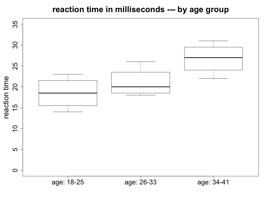
We begin by creating side-by-side box plots (Fig. 5.2.1).
It is also useful to calculate some summary statistics from the raw data (Table 5.2.2).
| Group | Sample Size | Sample Mean (ms) | Sample Variance |
| age 18-25 | 4 | 18.50 | 15.000 |
| age 26-33 | 4 | 21.00 | 12.667 |
| age 34-41 | 4 | 26.75 | 14.250 |
We can see that there appear to be some differences between the means of the three groups, particularly between the oldest and youngest. The oldest subjects (34-41) were about 8 ms slower responding to an audio stimulus compared to the youngest subjects (18-25) and almost 6 ms slower than people age 26-33. The youngest and intermediate age subjects however are only about 2.5 ms apart in mean reaction time. We would like to know — are any of these differences in mean response times statistically significant? We will also wish to ask if they are biologically meaningful.
We also note that the variances of the three groups do not appear to be greatly different. With such small sample sizes it is difficult to evaluate whether there may be a possible concern with the assumption of normality. However, since no strong skewness is apparent in Figure 5.2.1, there should not be a problem with using a method based on this assumption.
Model Formulation
Inference using the one-way model again relies on normal theory. Using notation similar to that used for the two independent-sample case, we can write
Equation 5.2.1 [latex]Y_{ij}\sim N(\mu_{i},\sigma_i^2)[/latex].
This reads that the jth observation in the ith group is distributed normally with a (population) mean of [latex]\mu_{i}[/latex] and a (population) variance of [latex]\sigma_i^2[/latex].
Another way of writing this model that will provide a notational framework for more complex models, is as follows:
Equation 5.2.2 [latex]y_{ij}=\mu +A_i+e_{ij}[/latex]
Here, [latex]y_{ij}[/latex] represents the reaction time for individual j in age group i, [latex]\mu[/latex] is an overall mean, [latex]A_i[/latex] is the effect of the ith level of age, (i=1,2,3), and [latex]e_{ij}[/latex] is called the error term. Here j=1,2,3,4 refers to the individual within each age group. We are replacing [latex]\mu_{i}[/latex] with [latex]\mu + A_{i}[/latex] in order to separate out a term that represents the age group. Also, in this model, the distributional assumptions are provided by the error term.
[latex]e_{ij}\sim N(0,\sigma^2)[/latex].
Assumptions for One-Way Model
Since the one-way model is the extension of the two independent-sample t-test to more than two groups, the assumptions are very much the same — but now must apply to 3 or more groups. We repeat them here. (Please refer to the section on the two independent-sample t-test for some added information, particularly for comments on robustness.)
(1) Independence:
The individuals/observations within each group are independent of one another and the individuals/observations in any one group are independent of the individuals/observations in all other groups.
(2) Equal variances
The population variances for each group are equal. (Similar conditions on robustness apply as in the two independent sample case.)
(3) Normality
The distributions of data for each group should be approximately normally distributed. (Similar conditions on robustness apply. The key is to avoid substantial skewness.)
Hypotheses for One-Way Model
The best way to write the statistical hypotheses is as follows:
Ho : all [latex]\mu_i[/latex] are equal
HA : not all [latex]\mu_i[/latex] are equal
For our reaction time example, the null hypotheses can be written
Ho : [latex]\mu_1 = \mu_2=\mu_3[/latex].
The alternative hypothesis only indicates that the (population) means of the groups are not all equal. All three means could be different or two could be the same and the third different. Support for the alternative from such a test provides no information as to how the means differ. We will have more to say about this later.
Comparison of “variability among group means” with “variability within groups” — Partitioning sums of squares
The basic idea is to compare the variability among the group (treatment) means with the variability within the groups. If the groups means are well spread out — and hence there is substantial among group variability — and this is large compared to the within group variability, this will provide evidence against the null hypothesis.
We illustrate this idea with the following two diagrams (using made-up data) that represent situations with 3 groups and 4 subjects per group.
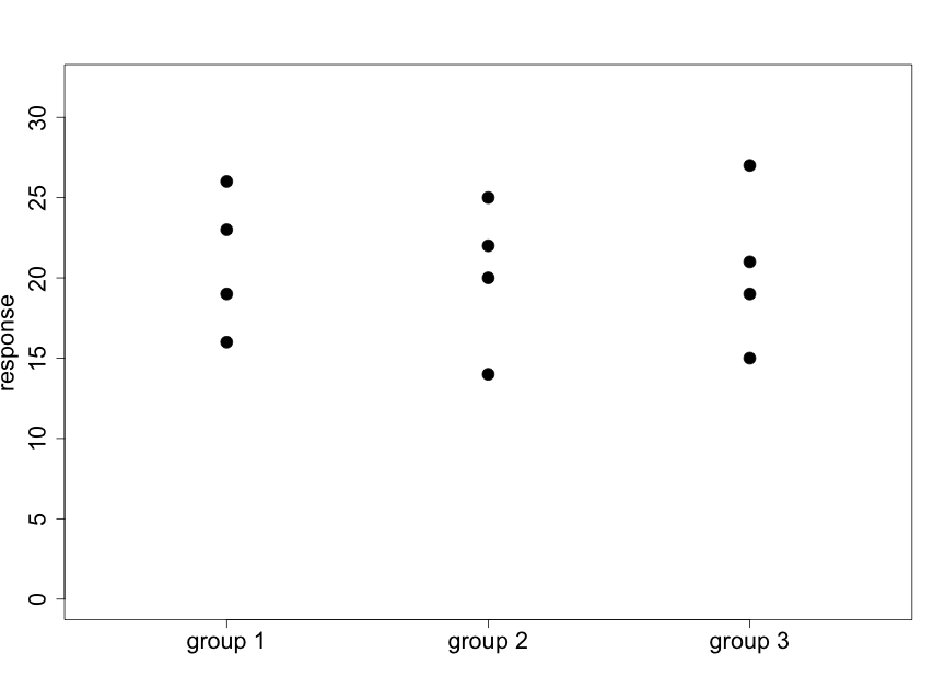
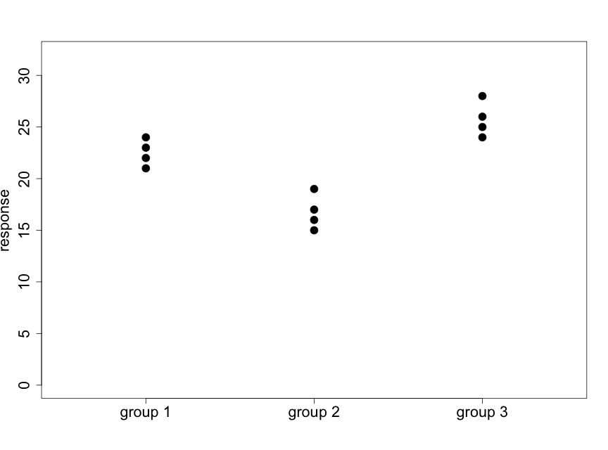
Fig. 5.2.2 illustrates a case where there appear to be very small differences among the means of the three groups relative to the variability within the groups. Data like these will support the null hypothesis. In Fig. 5.2.3 we see that the differences among the means of the three groups are large relative to the variability within the groups. Data like these will provide evidence against the null hypothesis.
Looking at the reaction time box plots above (Fig. 5.2.1), the reaction time data do not appear like Fig. 5.2.2 but they are also not as “extreme” as Fig 5.2.3. We will need to conduct the formal test to determine whether or not we reject the null hypothesis.
Computations for One-Way Model
We know that variances are a sum of squares divided by the appropriate degrees of freedom. The mathematical basis for the needed computations rests on the following:
total sum of squares = among groups sum of squares + within groups sum of squares
Note that the total sum of squares was defined near the beginning of this chapter. We will not provide detailed formulas for the other pieces but will obtain these from R. The primary output from such an analysis is an ANOVA table. Note!!! — This is where care is needed with the terminology. An ANOVA table can be produced for many models (including, for example, regression models). All ANOVA tables follow directly from the partitioning of the total sum of squares given in the formula just above. The one-way model is just one of many models for which an ANOVA table can be produced. Thus, the practitioner must be careful and recognize that the term ANOVA sometimes refers to a type of table (that can be produced for many models) and sometimes to a particular model (such as the one-way model for the reaction time example considered here).
Let us produce the ANOVA table that corresponds to the reaction time example and then explain all the parts. The R statistical program output would look something like the following. (Note that the output from the R commands does not include the line headed by “Total”. We have added this line here “for completeness”. The df and SS values on the “Total” line are the sum of the “Among groups” and “Within groups” values.)
We present the ANOVA output in a form that is commonly used for presentation.
| Source of Variation | df | SS | MS | F | p-value |
| Among groups | 2 | 143.17 | 71.583 | 5.12 | 0.0327 |
| Within groups | 9 | 125.75 | 13.972 | ||
| Total | 11 | 268.92 |
The “Source of Variation” indicates the category. Here, the “Total” is partitioned into “Among groups” and “Within groups”. The “SS” denotes sum of squares and “df” is our old friend degrees of freedom. The “MS” stands for mean square and is defined as follows:
[latex]MS = \frac{SS}{df}[/latex].
Thus, MS for “Among groups” is related to the variability among treatment means (although it should not be viewed directly as a formal variance). The MS for “Within groups” is the within treatment variance. We will discuss “F” and the associated p-value shortly.
By way of explanation, let us focus on the “Within groups” row. The value for the MS, 13.972, is an estimate of the underlying “within group” variance. Recall the way we formulated our model in eqn 5.2.1. Also, recall that we assume that the variances for each group have the same value. Thus, 13.972 is the estimate of the underlying [latex]\sigma^2[/latex]. Note the estimates of the variances within each group in the table of summary statistics. The value 13.972 is a weighted average of the individual variances where the weights are the df for each group, 3, 3, and 3 respectively. Also recall the definition for the pooled variance, [latex]s_p^2[/latex] from the last chapter. The “Within group” MS is just the extension of that equation to more than two groups. The df for “Within group” is just the sum of the df within each group. Thus, df (Within group) = 3 + 3+ 3 = 9.
There are three age groups in our reaction time example. The “Among group” df is just the number of groups minus 1. Thus, df (Among group) = 2.
Remember, the main idea in testing the null hypothesis that all group population means are the same is to compare the among group variability with the within group variability. We formalize this by means of the F test statistic:
[latex]F=\frac{MS_{among}}{MS_{within}}[/latex]
Under the null hypothesis, this F statistic is distributed according to the F distribution. Like the [latex]\chi^2[/latex]-distribution, it can only take non-negative values and the distribution is asymmetrical and has a “tail” to the right. However, the F is indexed by two different values for df: numerator df and denominator df. The among group piece is the numerator and the within group portion is the denominator.
Expand to see a sketch of the F-distribution for several different combinations of degrees of freedom.

(Interesting aside: The F-distribution is named in honor of R.A. Fisher, a British statistician from the first half of the 20th century who probably did more than any one else to bring the field of statistics to prominence. He also was a world-class quantitative geneticist.)
From the ANOVA table (Table 5.2.3) we see that the F-statistic value for the reaction time data is 5.12. The p-value can be written as [latex]p-value = Prob(F(2,9)\geq 5.12)[/latex]. Since the F-distribution is indexed by two distinct degrees of freedom, tables for it are structured somewhat differently than tables for the t and [latex]\chi^2[/latex] distributions. You enter the F-tables in the Appendix by finding the appropriate numerator and denominator df — 2 and 9 in this case. You can see that the 5.12 value is bracketed between 4.26 and 5.71. Thus, [latex]0.025 \lt p-value \lt 0.05[/latex].
Since we will be relying on statistical programs for ANOVA-type computations, we will almost always use the p-values that are part of the program output. For our example, the p-value is 0.0327. Thus, the null hypothesis is rejected at 5%. We know that the (population) reaction time mean for at least one of the age groups is different from the population means for the other two age groups.
(Although we will rarely if ever need to do so, R makes it easy to find the p-value given a value for the F-statistic and the degrees of freedom.)
The F statistic value will be large in magnitude when the among group variability (variability among treatment means) is large relative to the within group variability (within treatment variability).
Large within group sample sizes (and thus large within group degrees of freedom) will increase the ratio of the among group variability to the within group variability.
A large F statistic value leads to a small p-value.
Additional Comments
[1] More on Assumptions: —– A complete statistical analysis for the one-way model will include a careful assessment of the underlying assumptions. There are tools for doing this that go beyond what we can cover here. (These can be found in many of the better textbooks on statistics.) It is important to note that independence is always of great importance. To use the one-way model, it is necessary that there is no relationship between an observation on one group and an observation on any other. An evaluation of this — along with assessing whether or not the observations are independent within each group — depends most heavily an a careful consideration on the design and conduct of the study. Indeed, an awareness of the independence issue is critical at the planning stage of a study.
There do exist relatively good tests for determining if the variances are equal. (The Levene’s test is recommended.) However, as noted earlier, if the sample sizes for the various groups are similar in size, the formal inference is moderately robust to variance differences. (However, if you find that the sample variances differ by large amounts — say by a factor of 5 or more — then you may wish to consider other methods.) Finally, so long as the distribution of values within each group is not greatly skewed, there is considerable robustness against departures from normality.
Assumptions for One-Way Model
- Observations must be independent among groups and within groups
- Within group variances need to be the same (moderate robustness if sample sizes are close to the same for all groups)
- Within group data need to be normally distributed (the key is to avoid substantial skewness)
[2] Relationship between the F-test and the t-test with two groups: —– Even if there are only two groups, it is fully appropriate to use a one-way model. Now there will be 1 df for “Among group”. The results are fully consistent. In this case one can show— mathematically and empirically—that [latex]F = T^2[/latex]. Pretty neat, huh?
Section 5.3: After a significant F-test for the One-way Model; Additional Analysis
A conclusion of support for the alternative hypothesis in the one-way model does not provide any information about how the group means differ. It only indicates that the group population means are not all the same. For our reaction time data set, recall that the oldest subjects (age 34-41) had a mean that was about 8 ms slower responding to an audio stimulus compared to the youngest subjects (age 18-25). Is this difference statistically significant? How about the almost 6 ms difference between the (26-33) group and the oldest group?
There are many methods available for pursuing the issue of how the group means differ. Here we will focus on the protected t-test method. [Note — this method should be used ONLY IF our F-test leads to the rejection of the null hypothesis underlying the one-way model!!]
Suppose that we wish to focus on a threshold for significance of 5%. Then, if the p-value for the F-test (from the ANOVA table) is above 5%, we conclude that there are no differences among the group means and we do not make any further tests. Only if that p-value is less than 5%, do we proceed with a t-test. (This is the basis for the word “protected”.)
The protected t-test can be thought of as a two-independent sample test for all possible pairs of groups. We will use the procedure introduced in the previous chapter with some minor modifications. Let us index the two groups for a given comparison by i and j. Similar to eqn 4.2.1,
[latex]T=\frac{\overline{y_i}-\overline{y_j}}{\sqrt{s_p^2 (\frac{1}{n_i}+\frac{1}{n_j})}}[/latex]
Now, for [latex]s_p^2[/latex], we use the MS (mean square) from the Within groups line of the ANOVA table. We note that [latex]s_p^2=13.972[/latex]. Since an underlying assumption for the one-way model is that all group population variances are the same, we view the Within groups MS as our best estimate.
Let us now determine whether or not the population means from the 18-25 and 34-41 age groups are the same.
[latex]T=\frac{26.75-18.50}{\sqrt{13.972(\frac{1}{4}+\frac{1}{4})}}=3.121.[/latex]
The appropriate df for this are the df that go into the Within groups MS — 9 in this case. As before, we enter the t-tables using the proportion in two-tails. Thus, p-value < 0.01. (The exact p-value is 0.0061.) There is a very significant difference between the means of these two groups.
Let us now compare the 18-25 and 26-33 groups and also the 26-33 and 34-41 groups. Recall that the youngest (age 18-25) and intermediate (age 26-33) subjects had very similar average reaction times that are only 2.5 milliseconds apart, but the intermediate and oldest groups had a difference of almost 6 ms. Using exactly the same approach (but using the appropriate treatment mean values for each test) the resulting T-values are 0.946 and 2.175 respectively. For comparing the youngest and middle groups, we find 0.20<p-val<0.50 and for the intermediate and oldest groups, 0.05<p-val<0.10. Thus there is not enough evidence to conclude that the population means for the 18-25 and 26-33 groups or for the 26-33 and 34-41 groups differ significantly at 5%, although one could say that there is some marginal evidence that the intermediate and oldest groups are not the same.
Reporting results from a one-way model analysis:
The first step is to fully describe the design and conduct of the study. This is to ensure that the reader will be certain that the “analysis follows the design”. Explicitly identify the groups and provide the sample size for each group. Provide the F- and p-values along with the underlying degrees of freedom. (It is often sound practice to report the Within group MS in order to provide an estimate of the underlying error variance.) It is important to Indicate that you have examined the assumptions and found no major violations. If you perform follow-up protected t-tests, make explicit that this is valid and provide a table with group means and an indication of significance.
For the reaction time example, Table 5.3.1 is a summary table of a form that is frequently used. Groups that share the same letter are non significantly different from one another.
| age group | sample mean (ms) | significance indicator |
| 18-25 | 18.5 | a |
| 26-33 | 21.00 | ab |
| 34-41 | 26.75 | b |
Since the first and second groups both have the letter “a”, they are not statistically significantly different. Similarly, the second and third groups do not differ significantly since they both have the letter “b”. However, the first and third groups are significantly different since they do not contain a common letter.
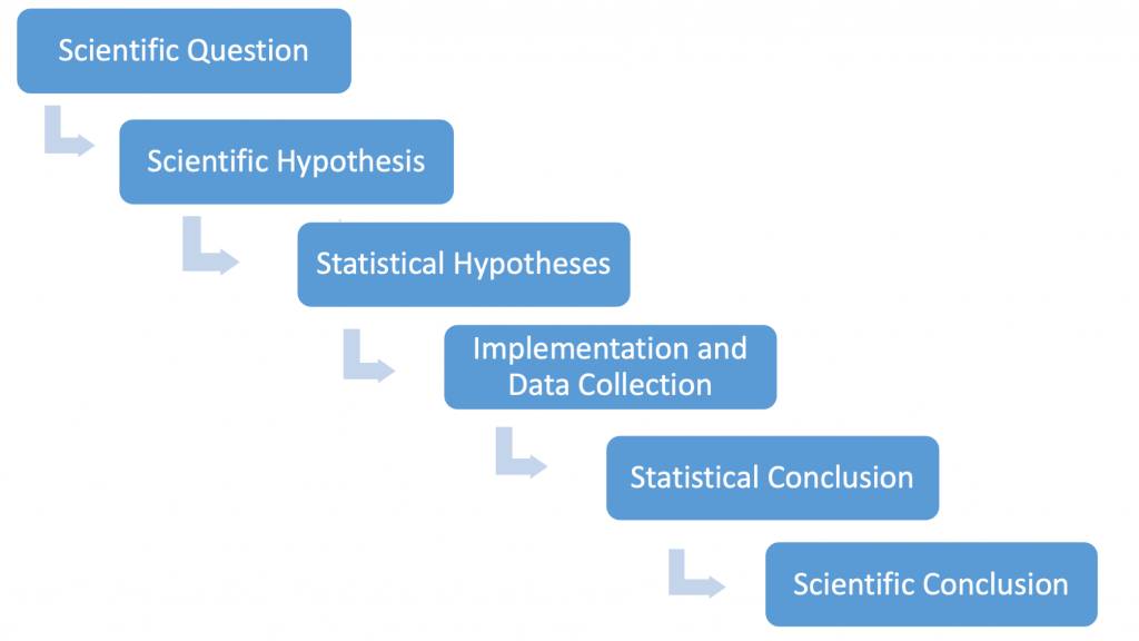
Recall our diagram of the logic connecting biology and statistics in hypothesis testing.
In the “Results” section of a paper or poster, here is how a scientist might summarize the results from the complete analysis of the reaction time data:
“In comparing the reaction times between three age groups: 18-25, 26-33, and 34-41 in a study with four subjects per age group, the null hypothesis that the mean times were all the same was rejected at 5% (F (2,9) = 5.12, p = 0.033). A follow-up protected t-Test indicated that the only significant difference in mean reaction times was the 8.25 ms difference between the youngest and oldest subjects (T (T(9) = 3.12, p=0.0061, two-tailed). The sample means for the 3 groups were: 18.5 ms (18-25); 21.0 ms (26-33); and 26.75 (34-41).”
Section 5.4: The Two-way Model
Scientists often study the effects of two (or more) different factors (e.g. experimental conditions, groupings of subjects, etc.) on a response (dependent) variable. Here we consider an example with two factors. This is sometimes referred to as a two-factor design and the appropriate model for analysis is the two-way model. It is important to recognize that this model is a further extension of the two-independent sample design. There must be independence among all combinations of treatment factors as well as within factors. (We will see later that there can be designs that are extensions of a paired design that bear some resemblance to the two-way model. These are referred to as blocked designs and need to be viewed as distinct from the two-way model.)
The data presented above on reaction time for young adults are actually a portion of a larger study. The previous data were obtained on young adults raised in urban environments. At the same time, similar data were also obtained on those raised in rural environments. A scientist might be curious about whether the environment has any impact on reaction time, and if so, whether this environmental influence is age-dependent.
Table 5.4.1 contains the complete data set.
Urban
| Reaction Time (age 18-25; ms) | Reaction Time (age 26-33) | Reaction Time (age 34-41) |
| 17 | 19 | 28 |
| 23 | 26 | 22 |
| 14 | 18 | 31 |
| 20 | 21 | 26 |
Rural
| Reaction Time (age 18-25; ms) | Reaction Time (age 26-33) | Reaction Time (age 34-41) |
| 17 | 22 | 27 |
| 13 | 27 | 33 |
| 22 | 21 | 24 |
| 19 | 17 | 30 |
Again, we provide some useful summary statistics (Table 5.4.2).
| Group | Sample Size | Sample Mean (ms) | Sample Variance |
| age 18-25: urban | 4 | 18.50 | 15.000 |
| age 18-25: rural | 4 | 17.75 | 14.250 |
| age 26-33: urban | 4 | 21.00 | 12.667 |
| age 26-33: rural | 4 | 21.75 | 16.917 |
| age 34-41: urban | 4 | 26.75 | 14.250 |
| age 34-41: rural | 4 | 28.50 | 15.000 |
Here, it makes sense to introduce a new kind of plot. In this figure, the x-axis will denote the age group and the y-axis will indicate the reaction time. There will be separate points (and lines) on the plot for each background environment. Figure 5.4.1 shows a plot of the means of each group of four observations.
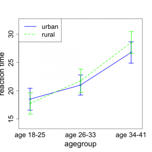
We note that the mean reaction time goes up with age group for subjects living in both rural and urban environments. It appears that the increase may be slightly greater for those from rural backgrounds than for those from urban environments.
This type of plot is often referred to as an interaction plot. It allows us to determine to what extent the relationships between age group and mean reaction time are the same or different between the two environments. If the general shapes of the lines are parallel, this suggests that the patterns of increase are the same for the two environments. Lack of parallelism suggests that the increases in patterns differ and hence there is interaction between environment and age. This would signify that the effect of age on reaction time is different for the two different environmental groups. In many instances, identifying a significant interaction is a very important scientific finding. The plot in Fig. 5.4.1 indicates there may be a hint of non-parallelism; however, we will need to conduct formal inference to determine if the interaction between age and environment is significant or not.
The Two-way Model and Assumptions
Before providing an analysis of these data, let us briefly describe the underlying model and assumptions. Building on the notational framework introduced in equation (5.2.2), we can write this model as follows.
[latex]y_{ijk}=\mu +A_i+E_j+AE_{ij}+e_{ijk}[/latex]
Here, [latex]y_{ijk}[/latex] represents the reaction time for an individual, [latex]\mu[/latex] is an overall mean, [latex]A_i[/latex] is the effect of the ith level of age, (i=1,2,3), [latex]E_j[/latex] is the effect of the jth level of background environment, (j=1,2) [latex]AE_{ij}[/latex] is the interaction term, and [latex]e_{ijk}[/latex] is called the error term. Here k=1,2,3,4 refers to the individual within each combination of age and background. Again, assuming normal theory,
[latex]e_{ijk}\sim N(0,\sigma^2)[/latex].
As in the one-way model, [latex]\sigma^2[/latex] is the underlying population variance. As before, we will estimate this with the mean square for error.
The basic assumptions are the same as with the one-way model (with some technical modifications) but we now add a fourth assumption, which we place first in the list below. This assumption has been implicit for all previous models.
(1) Correct Model:
The model used for analyzing the data is consistent with the design and implementation of the study. (Suppose with the current example with two environments and three age groups, we used a model for analysis that assumed a pairing between subjects from the two environments. This would NOT be the correct model and would almost certainly lead to inappropriate conclusions.)
(2) Independence:
The individuals/observations within each treatment combination group are independent of one another and the individuals/observations in one group are independent of the individuals/observations in all other groups.
(3) Equal variances
The population variances for each group are equal. (Similar conditions on robustness to those noted earlier apply.)
(4) Normality
The distributions of data for each group should be approximately normally distributed. (Similar conditions on robustness apply.)
There are now three statistical hypotheses of potential interest to the researcher. (We will only state the null hypothesis here since the alternative will always be that the null is not true.)
Ho1 : all [latex]A_i=0[/latex] — there are no differences among the means of the three age groups (with data averaged over environment). In other words, this null hypothesis states that mean reaction time is the same for all age groups, averaging over the environments.
Ho2 : all [latex]E_j=0[/latex] — there is no difference between the means of the two environments (with data averaged over age groups). In other words, the mean reaction time is the same for both environments, averaging over the age groups of subjects.
Ho3 : all [latex]AE_{ij}=0[/latex] — there is no interaction between age group and environment. In other words, any effect of age on reaction time is not influenced by subjects’ environment (rural or urban), or vice versa.
We will provide additional interpretation to these null hypotheses after presenting the analysis of variance table.
Again, we will provide the output (Table 5.4.3) from the R package and avoid the algebra associated with the detailed computations. Information on the computational details can be obtained from many standard statistics textbooks. (Again, we include the “Total” row for which the listed values are just the sum over the previous 4 rows.)
| Source of Variation | df | SS | MS | F | p-value |
| Age | 2 | 373.00 | 186.50 | 12.70 | 0.00036 |
| Environment | 1 | 2.04 | 2.04 | 0.14 | 0.71 |
| Age*Envir interaction | 2 | 6.33 | 3.17 | 0.22 | 0.81 |
| Error | 18 | 264.25 | 14.68 | ||
| Total | 23 | 645.62 |
Since there are 3 age groups, there are 2 df for age. Similarly, there is 1 df for environment. The df for the interaction is the product of df age and df environment. That is 2 in this case. Since there are 24 total observations, there are 23 df for the total. The df for error can be calculated as 23 minus the sum of the df for the previous sources. Thus 18 = (23 – 2 – 1 – 2). Another way to think of the df for error is as follows. Within each treatment combination group, there are 4 observations. This means that each group contributes 3 df towards estimating the error variance. Since there are 6 groups, 3 * 6 = 18.
The p-values in the last column are the results of the tests of the three null hypotheses listed above. In this case, the null hypothesis of no age effects is very strongly rejected (p-value = 0.00036). Thus, there are large mean reaction time differences among age groups, averaged over environment. However, there is no evidence against the null of no environment effect (p-value = 0.71) and the null of no interaction (p-value = 0.81). Although the interaction plot hinted at some potential interaction (non-parallelism), the formal test demonstrates that the lack of parallelism can easily be explained as “random noise”. The plot clearly suggests that there is no environment effect. The age effect is very clear.
It is important to say a bit more about the test for interaction. Suppose that the null hypothesis of no interaction is rejected. This means that the effect of one factor on the response is different for different levels of the other factor. This clearly suggests that both factors have a significant impact on the data. This is true even if the “main effect” for one factor — looking at differences for that factor when the data are averaged over the other factor — is not significant. Thus, suppose that in our example, there was significant interaction but that the null hypothesis Ho2 was not rejected. It would not be correct to say that environment was not significant. The significance of the interaction says that the effect of environment on reaction time is significantly different for different age groups — even if there is no significance in environment averaged over age group.
Section 5.5: Analysis of Variance with Blocking
Reconsider the heart rate example illustrating a (two-sample) paired study described previously. In that example the goal was to compare the heart rate for students between a resting state and stair-climbing. Each student had their heart rate measured under each of the two conditions. Inference was conducted on the difference in heart rates.
Suppose that scientists wished to expand the study by including a different type of exercise (e.g., a 40 meter sprint). In this case there would be a three conditions under which student heart rate would be measured: resting state, stair-climbing, and running 40 meters. This leads to a different design, the extension of the paired design to more than two treatments. Such designs are called blocked designs. In this example the blocks are the individual students. Data are obtained for each condition (resting, stair climbing, running 40 meters) for each student.
In the first chapter, we described randomized block sampling. Recall the importance of randomizing the treatments to “plots” within each block to avoid possible biases. For situations like the current three treatment heart rate study, we need to randomize the order in which each individual student encounters each activity — resting, stair climbing, running 40 meters. We would need to ensure that there was adequate rest time between activities so that a student’s response to a given activity will not be impacted by a previous activity (perhaps by fatigue). In practice, order randomization may not always be possible. However, if the time between activities is large enough to avoid any impact of an earlier activity on a later one, it may be safe to use the method of analysis described here — even without order randomization.
The appropriate method of analysis for blocked designs leads to a different “ANOVA-type” model. The model can be written
[latex]y_{ij}=\mu +C_i+B_j+e_{ij}[/latex]
Here, [latex]y_{ij}[/latex] represents the heart rate for individual j under condition i, [latex]\mu[/latex] is an overall mean, [latex]C_i[/latex] is the effect of the ith condition, (i=1,2,3), [latex]B_j[/latex] is the effect of the jth block — the individual, (j=1,2,…J) where J is the total number of individuals, and [latex]e_{ij}[/latex] is called the error term. Again, assuming normal theory,
[latex]e_{ij}\sim N(0,\sigma^2)[/latex].
The same four basic assumptions underlie this model: correct model, independence, equal variance, and normality. However, the “correct model” assumption includes the following. The effects of treatment (condition) and block (individual) are additive. This means that if there is a block (individual student) effect, it is the same for all conditions!! (Another way of thinking about this is that there must be no interaction between treatment and block.) For the heart rate study, the additivity assumption means that the difference in heart rate between any two individuals needs to be the same for all three activities. Thus, even though the average condition for students may vary, the change in heart rate from one activity to another needs to be (on average) the same for all students.
If the assumption of additivity is not met, then we must conclude that the correct model assumption is not satisfied and the model given above is not appropriate. It is beyond the scope of this primer to discuss this assumption further. However, it is strongly suggested that a plot, like the interaction plot described above, be created — with separate “lines” for each block. In order for the additivity assumption to hold, the lines should not indicate too strong a departure from parallelism.
There may appear to be some similarity between the model for the blocked design and the one for the two-factor design discussed in the previous section. One might think that the blocked design is the same as the two-model design without the interaction. The way models are written can obscure the underlying design. The key is the actual design used for conducting the experiment. In the blocked design the blocking factor (individual for the heart rate example) is NOT a treatment factor and is used only to reduce the variability for assessing the impact of the experimental treatment (exercise regime). Thus, even though the “models” may appear similar the designs are different. The analysis and the interpretation must take this into account.
We will not further develop this heart-rate example here. However, blocking is included in the example in the following section and a complete analysis will be provided.
Section 5.6: A Capstone Example: A Two-Factor Design with Blocking — with a Data Transformation
Let us now consider a more complex example that contains many of the elements we have described. Suppose students in a cell biology lab are asked to design a novel experiment using eukaryotic yeast as a model system to study cellular signal transduction. The students are encouraged to design a research project involving two independent variables, the presence/absence of alpha factor (a mating pheromone) and a treatment such as different environmental temperatures or drug dosages. The students use a beta-galactosidase reporter assay to measure yeast mating gene transcriptional activity.
Continuous data such as those collected from the beta galactosidase enzymatic assay are best analyzed using ANOVA methods. Imagine that you hypothesize that yeast mating gene transcription in the presence of alpha factor is dependent on environmental temperature. Specifically, you hypothesize that in the presence of alpha factor, the beta galactosidase activity (measured in Miller units) in “a” type cells will increase as the temperature increases from 22 to 37ºC, as compared to “a” cells with no alpha factor exposure at these temperatures. Here we have 2 independent (“predictor”) variables (environmental temperature and alpha factor presence) and one continuous dependent variable (mating gene transcription as measured by beta-gal activity).
This information by itself is not sufficient to determine the proper method of analysis. It is necessary to fully understand the way the experiment was conducted. The procedure was as follows. A 1/4 loop of yeast (taken from colonies of yeast growing on nutrient agar plates) was placed in a flask with 20ml of broth and allowed to grow overnight. The next day, 3.3ml from the overnight flask were placed in another flask with 26.7 ml of additional broth. (This is a dilution step.) Five flasks were prepared in this step. We will refer to these 5 flasks as replicates or “reps”.
After two hours, four aliquots were taken from each rep and placed in separate test tubes. The four treatment combinations: +alpha/22ºC, -alpha/22ºC, +alpha/37ºC, and -alpha/37ºC were randomly assigned to the four test tubes — with the randomization done independently for each rep. Thus, there are a total of 20 test tubes.
This design is one with two factors (experimental treatments), but also with blocking. The reps (flasks) are blocks. Despite the most careful experimental procedure, it is possible that each of the 5 reps may be somewhat different. (Perhaps the dilution varies somewhat from rep to rep.) Thus, each of the 4 test tubes obtained from a single rep (flask) will be affected similarly by the particular content of that flask, and so there is a potential relationship between one observation within a rep and another. This is the essence of blocking. The rep (dilution flask) is the blocking factor in the same way that student was in the heart rate example.
It is entirely possible that the experiment could have been conducted in a different way that would not be considered as a blocked design. Suppose that, instead of preparing 5 flasks, we prepared 20 flasks. Suppose further that we took only a single aliquot from each of the 20 flasks and placed it in a test tube and that each of the four treatment combinations was randomly assigned to 5 of the test tubes. We again would have 20 test tubes — but now they would all be considered independent of each other. Thus, the design would be correctly described as a simple random design. The analysis would follow that of the two-way model (with no blocking). Remember, analysis follows design.
The observed data are presented in the following form in Table 5.6.1.
| TREATMENT | ||||
REP |
+alpha/22ºC | -alpha/22ºC | +alpha/37ºC | -alpha/37ºC |
| 1 | 1600 | 210 | 3100 | 140 |
| 2 | 1800 | 270 | 3500 | 240 |
| 3 | 2100 | 140 | 3700 | 260 |
| 4 | 1900 | 160 | 3600 | 130 |
| 5 | 2000 | 250 | 3300 | 240 |
As always, it is important to plot the data. In Figure 5.6.1, we use a plotting procedure that allows the effects of the two factors and the reps to be visualized.
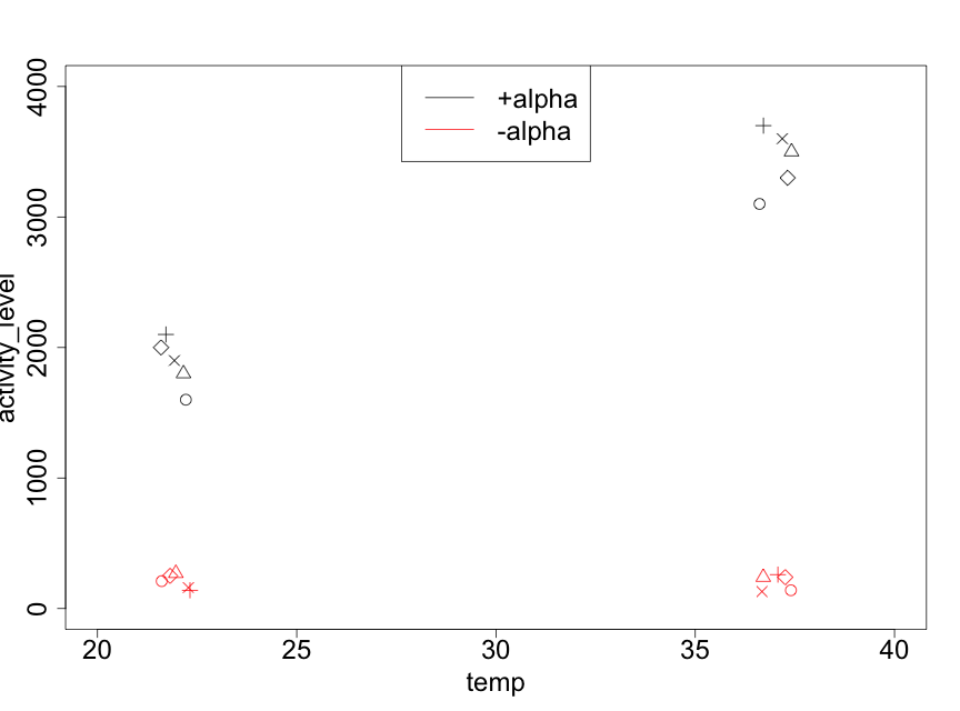
It is immediately clear that the mating gene transcription activity levels are substantially larger for the +alpha treatments than for the -alpha ones. We also note that, as the temperature changes from 22ºC to 37ºC, the -alpha data have similar values whereas the +alpha data show an increase. The fact that the effect of temperature is different for the two levels of alpha factor (or, equivalently, that the effect of alpha factor on mating gene transcription is different for the two levels of temperature) indicates that there is an interaction between the two experimental factors. We will see if this is indeed statistically significant.
We also note that it appears that the effect of reps is quite modest. Nonetheless, since the experiment was conducted with reps, this must be taken into account in the analysis. However, the plot does indicate that the variances for the 4 treatment combinations appear to differ. In particular, the larger the mean (of the 5 data points for a given treatment combination), the higher is the variance. Table 5.6.2 makes this clear.
| treatment combination | mean (Miller units) | variance |
|---|---|---|
| +alpha/22ºC | 1880 | 37000 |
| -alpha/22ºC | 206 | 3130 |
| +alpha/37ºC | 3440 | 58000 |
| -alpha/37ºC | 202 | 3820 |
In Sec 4.3 we presented a two-independent sample example with assumption violations. In that example the variances were quite unequal. The group with the larger mean had the larger variance. That was one of the indications (for that example) that a transformation was needed. In that case a log transformation was a sensible one.
Data from biological studies often show a pattern where the variance increases with the mean. However, a log transformation is not always the most appropriate. By empirical evaluation (trying various transformations for the beta galactosidase data), we find that a square root transformation does a good job of equalizing variances. (As noted earlier, with biological data, the log and square root transformations are the most commonly used.)
In studies such as this example of measuring gene transcriptional activity via a beta galactosidase assay, we do not have enough data per treatment combination to assess normality. An examination of the square root transformed data reveals no obvious problem with skewness.
Using the transformed data, we first reproduce the data table (Table 5.6.3) and the mean-variance table (Table 5.6.4).
| rep \\ trt | +alpha/22ºC | -alpha/22ºC | +alpha/37ºC | -alpha/37ºC |
|---|---|---|---|---|
| 1 | 40.00 | 14.49 | 55.68 | 11.83 |
| 2 | 42.83 | 16.43 | 59.16 | 15.49 |
| 3 | 45.83 | 11.83 | 60.83 | 16.12 |
| 4 | 43.59 | 12.65 | 60.00 | 11.40 |
| 5 | 44.72 | 15.81 | 57.45 | 15.49 |
| treatment combination | mean | variance |
|---|---|---|
| +alpha/22ºC | 43.31 | 5.034 |
| -alpha/22ºC | 14.24 | 3.916 |
| +alpha/37ºC | 58.62 | 4.277 |
| -alpha/37ºC | 14.07 | 5.098 |
We see that, using the transformed scale, we no longer have a problem with unequal variances. Thus, we have found a scale in which the assumptions are met and we can proceed with our inference on this scale.
We now provide an interaction plot (Figure 5.6.2) of the transformed data. For this plot, we take the mean over the 5 reps for each treatment combination and provide a plot similar to that we presented for the two-way model example on reaction time.
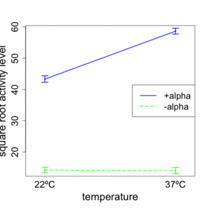
We note from the plot that the general nature of the interaction is not changed (compared to Fig 5.6.1). With -alpha, we see that the square root of mating gene transcription activity does not change much with temperature. However, for +alpha, the response increases notably with temperature. Thus, the effect of temperature on mating gene transcription is different for +alpha and -alpha; this is a clear indication that there is an interaction between temperature and alpha factor.
We now generate the analysis of variance table (Table 5.6.5) using the square root of the activity levels as the response.
| Source of Variation | df | SS | MS | F | p-value |
| Reps | 4 | 28.7 | 7.2 | 1.93 | 0.170 |
| Alpha Factor | 1 | 6775.5 | 6775.5 | 1823.7 | 1.8*10-14 |
| Temperature | 1 | 286.3 | 286.3 | 77.1 | 1.4*10-6 |
| Alpha*Temp interaction | 1 | 299.7 | 299.7 | 80.7 | 1.1*10-6 |
| Error | 12 | 44.6 | 3.7 | ||
| Total | 19 | 7434.8 |
The first p-value we examine is the one that corresponds to the interaction term. This is highly significant (p-value = 1.1 x 10⁻⁶). Thus, even if the p-values for Alpha Factor and Temperature were greater than 0.05, we would conclude that both alpha factor and temperature are very important. Since the “main effects” for Alpha Factor and Temperature both have very small p-values (1.8 x 10⁻¹⁴ and 1.4 x 10⁻⁶, respectively), we see that we strongly reject all three of the null hypotheses: (i.e., the null hypotheses that there is [1] no average alpha factor effect, [2] no average temperature effect, and [3] no interaction between temperature and alpha factor.
An examination of the plot (Fig. 5.6.2) clearly supports the statistical results. The responses for +alpha are very much larger than for -alpha — for both temperatures. The average responses (across the two alpha factor levels) at 37ºC are considerable higher than at 23ºC. Also, the two lines deviate substantially from parallelism, thus indicating strong interaction. For -alpha, there appears to be no meaningful effect of temperature on mating gene transcription activity. (A formal test of the significance of this requires steps beyond those that we provide here.) For +alpha, the mating gene transcription activity level increases markedly with temperature.
Although it is generally not considered good statistical practice to attach any formal statistical meaning to the p-value for reps, we can see that the very small F-value (and correspondingly moderately large p-value) for reps suggests that there were no meaningful average differences among the reps. For the yeast experiment described above, this indicates that the “rep” flasks did not have any notable influence on the mating gene transcription response. This provides useful information about the consistency of the implementation of our experiment; however, it is “best practice” to maintain this “rep” term in the ANOVA table.
Thus, we conclude that both temperature and presence or absence of alpha factor are highly significant in explaining the yeast mating gene transcription activity level (as measured in Miller units). In particular, the addition of the alpha factor pheromone greatly increases mating gene transcription activity level. On average, temperature is significant but this is primarily due to the increased effect of +alpha at 37ºC compared to 23ºC. This difference in +alpha at the two temperatures gives rise to the significant interaction. Thus, we can state that the effect of alpha factor on mating gene transcription is indeed different at the two temperatures. It is significantly stronger at 37ºC than at 23ºC.
Describing the results of the Yeast Signal Transduction Example
Here are two paragraphs that would be useful for describing the analysis of the mating gene transcription study. This first paragraph describes the statistical methodology used and so would be appropriate for the “Methods” section of a scientific paper or poster:
“The underlying experimental design is one with two independent factors — alpha factor and temperature — and with blocking. From initial plots of the response — mating gene transcription activity level — it was found that the variance increased with the mean mating gene transcription activity level. A square root transformation removed the variance problem. A two-way model with blocking was fit to the square root transformed data. F-tests were conducted to test the null hypotheses of no interaction between alpha factor and temperature, no main effect for alpha factor, and no main effect for temperature.
The immediately following paragraph provides an example of how to summarize the statistical output from the Two-Factor ANOVA analysis. This paragraph would be appropriate for the “Results” section of a scientific paper or poster.
“The main effects for alpha factor and temperature, as well as the interaction between alpha factor and temperature were all highly significant (p-values: 1.8*10-14; 1.4*10-6; and 1.1*10-6 respectively.) For -alpha, the mean values for the square root of mating gene transcription activity (measured in Miller units) were similar for both 22ºC and 37ºC. However, for +alpha, the mating gene transcription response increased strongly from 22ºC to 37ºC.”
Section 5.7: An Important Warning — Watch Out for Nesting
Whenever studies are conducted with two experimental factors, it may be tempting always to analyze them as a two-way ANOVA with or without blocking. However, this can lead to major errors. With two (or more) experimental factors, there is a substantial range of possible designs. Some of these may lead to analyses like those considered above: reaction time (with factors age and environment) and mating gene transcription activity level (with factors alpha factor and temperature and also with reps as blocks).
However, consider the following. In Section 1.2 we discussed some study designs for determining whether the heights of Canada thistles in a field were affected by whether or not a field was burned. Imagine that we might wish to consider another experimental factor: the presence or absence of a mild weed killer.
Suppose that the field is divided into 6 sub-fields. Three randomly selected sub-fields are burned and the other three are not burned. Each sub-field is further divided into two halves (plots). Using proper randomization, one plot within each sub-field receives the mild weed killer and the other half does not. This design can be depicted schematically as shown in Figure 5.7.1:
| SF1: Burn
no wk |
SF1: Burn
wk |
SF2: No-Burn
wk |
SF2: No-Burn
no wk |
| SF3: No-Burn
wk |
SF3: No-Burn
no wk |
SF4: No-Burn
no wk |
SF4: No-Burn
wk |
| SF5: Burn
wk |
SF5: Burn
no wk |
SF6: Burn
wk |
SF6: Burn
no wk |
Figure 5.7.1: Example of a nested design. The dark lines delineate the 6 sub-fields (SF); the lighter lines separate the two halves (plots) of each sub-field. wk=weed killer.
We designate sub-field i as SFi where i ranges from 1 to 6. There are 12 plots in this study. Each of the two plots within a sub-field have the same burning treatment. Thus, the impact of the burning treatment affects both plots in a similar fashion. Any plot within a sub-field will have some “dependence” on the other plot within the same sub-field that it will not have with any plot in another sub-field. We say that the weed killer treatment is nested within each sub-field. Because of this nesting, an analysis using the ANOVA table for the two-way model — like the one we used for the reaction time example — would be incorrect. The proper analysis is more complicated and beyond the scope of this primer. It can be found in more advanced textbooks.
All scientists need to be on the lookout for nesting in the design of their studies. The failure to account for nesting is, perhaps, the most common error that scientists make in analyzing experimental data.
Section 5.8: A Brief Summary of Key ANOVA Ideas
Many scientific studies lead to analyses of the effects of multiple factors and factors with two or more levels. With quantitative data, there is a very large number of statistical models that can be used for such analyses. However, substantial care is necessary to ensure that the right model is chosen for each particular experimental design.
All models appropriate for such analyses share the same four basic assumptions, which we state in a useful “short form” below. However, different designs require different ways of thinking about Assumption #1.
The correct model assumption states that the analysis must follow the design. We have seen in many of the above examples that different designs require the data analyst to focus on different specific issues. For example, understanding whether a design has blocking — or not — is necessary for selecting the correct model. As another example, in a design with blocks, the correct model assumption requires that the blocks are additive with the treatments. (See the discussion earlier in the chapter for more information on this.). A further example is the occurrence of nesting, as described in the previous section!!
In some cases there may be certain plots that can be useful for assessing the correct model assumption. However, the primary way to evaluate the assumption is by paying careful attention to the design and conduct of the study. This assumption is extremely important. If you do not choose the correct model, your analytical results will very likely be erroneous.
The independence assumption basically requires that the random variation in any given data point has no impact on the random variation of any other data point. If, for instance, your response variable is the height of a plant, the selection of two plants that are growing very close together would likely violate this assumption. If one plant is tall, it might be shading the second plant, thus impeding its growth. As with the correct model assumption, paying careful attention to the design and conduct of the study is key, and a violation of the independence assumption will very likely lead to erroneous results.
The equal variance assumption requires that the variances need to be the same for all combinations of treatments and blocks. Careful plotting of the data, for example see Fig. 5.6.1, can sometimes be helpful for assessment. There do exist some specialized procedures; however we will not pursue those here. There is modest robustness against departures from the equal variance assumption (i.e. modest departures can be tolerated) for data that are balanced or close to it. (Data are balanced if there are an equal number of observations for all combinations of treatments, blocks, etc..) In practice, data transformations — such as square root or log — are often useful to reduce problems due to non-constant variance. As noted, the need for transformations is quite common with biological data.
The normality assumption requires that the distribution of the random variation terms are normal. Note: this does not mean that the raw data looked at all together must be normal! There are a number of techniques, graphical and otherwise, for assessing this assumption. However, as noted several times earlier in the primer, the key concern is to avoid substantially skewed data. Histograms or stem-leaf plots can be useful in assessing skewness; however, with many complex designs, other techniques may be needed. The analytical procedures are quite robust to non-normality, so long as there is no substantial skewness.
A primary technical feature of ANOVA-type analysis is the idea of partitioning sums of squares. The idea is for each component (of the partitioning) to represent an important feature of the design so that the magnitude of the component’s effect on the dependent variable of interest can be compared to some measure of underlying variability. The basic ideas were described in Sec. 5.2.
