
Biocore Statistics Primer
Chapter 6: Further Analysis with Categorical Data
Section 6.1: Different Goals with Chi-squared Testing
In Section 3.3, we presented a brief introduction to a one-sample chi-squared test from genetics. In Section 4.5, we provided a two-sample example in which we compared the germination rates for hulled and dehulled seeds for a prairie forb. Both analyses were based on a chi-squared testing procedure. The ideas behind such tests can be extended to a substantially broader class of inference problems. The goal of the current chapter is to expand and generalize the discussion.
It is important to recognize a distinction between two types of scientific situations. In the dihybrid cross example from Chapter 3, we wished to determine whether or not our experimental results were or were not consistent with well-established theory strongly supported by the scientific literature. In such cases there are clearly established expectations for the pattern of data. For such studies we wish to determine if the observed data fit well — hence called goodness-of-fit tests — to the established expectations.
In many other scientific situations, scientists wish to know whether or not the proportions of observations in various categories are the same or not between (among) two (or more) groups. Here there typically is no existing literature that would provide, a priori, expected proportions. The goal now is to compare categorical proportions in two or more groups. Tests of this type are sometimes called homogeneity tests or tests of independence. Here we will not distinguish between these. You will see that the statistical analysis requires us to compute “expected values”. However, these expected values are not based on the scientific literature but on a statistical null hypothesis that the proportions of observations from each group are the same across all the categories.
The (one-sample) dihybrid cross example from Section 3.3 is an example for which a goodness-of-fit test is appropriate. We had two unlinked autosomal genes that affect seed characteristics, with two alleles at each locus and complete dominance in both cases. (“Round” is dominant over “wrinkled” and “yellow” is dominant over “green”.) For data in the F2 generation, we would expect ratios of 9 – 3 – 3 -1 in seed characteristics. Thus, there is underlying theory to suggest what the expected values should be — if the theory holds for the current example. Our goal is to determine if the observed data are consistent with the expected ratios. We produce again the observed data:
| round and yellow | 218 |
| wrinkled and yellow | 80 |
| round and green | 72 |
| wrinkled and green | 30 |
| total | 400 |
For the comparison of germination rates example, the test to be conducted can be thought of as a test of homogeneity. There is no prior body of literature suggesting what the germination rate for seeds from a prairie forb should be. The goal of the study was to determine if there was a difference (or not) between hulled and dehulled seeds.
In section 4.5 where we analyzed this example, we indicated that the number of seeds that germinated could be described by a binomial distribution. (There were exactly two categories for each seed: germinated or not.) For the dihybrid example, there are exactly four categories. The type of distribution used to describe this situation is the multinomial. We will say a bit more about this distribution in the next section when we discuss assumptions.
Section 6.2: The One-Sample Chi-squared Test
Before proceeding with further discussion of the dihybrid-cross example, let us re-emphasize that these data are categorical. Each observed seed belongs to a category (e.g. round and yellow). There is a numerical aspect to such data and that is the count. This count is just the number of observations in each category.
If we label the categories 1, 2, 3, and 4 and let [latex]p_i[/latex] represent the proportion of seeds in category i, we can write the null and alternative hypothesis underlying our study as follows.
H0 : [latex]p_1 = 9/16; p_2 = 3/16; p_3 = 3/16; p_4 = 1/16[/latex]
HA : not H0
The alternative indicates that the seeds do not follow the 9 – 3 – 3 – 1 ratios but does not provide any information about how the ratios might differ.
Here we are looking at a single sample and and intend to compare the observed data with what would be expected if the null hypothesis is true. With a multinomial distribution, if the null is true, we expect the proportions of observations in each of the four categories to follow the 9 – 3 – 3 – 1 ratios for the F2 generation in an unlinked, autosomal dyhybrid cross. As noted, this test is referred to as a goodness-of-fit test.
Based on the genetic principle of complete dominance, we expect that the 400 seeds will be distributed in concordance with the expected ratios. For example, with the round and yellow category, the expected number is 225 = (400 * 9/16). The full table of expected values is given in Table 6.2.1.
| round and yellow | 225 |
| wrinkled and yellow | 75 |
| round and green | 75 |
| wrinkled and green | 25 |
| total | 400 |
We calculate [latex]X^2=\sum_{all cells}\frac{(obs-exp)^2}{exp}[/latex].
[latex]X^2=\frac{(218-225)^2}{225}+\frac{(80-75)^2}{75}+\frac{(72-75)^2}{75}+\frac{(30-25)^2}{25}=1.671.[/latex]
Since we are dealing with the multinomial distribution with 4 categories, the degrees of freedom are the number of categories minus 1 — or 3 — in this case. We calculate a p-value as before, again using the chi-square table. Our observed value of 1.671 falls below the tabled value of 6.25 in the row with 3df. Thus, p-val>0.10. (The true p-value is actually 0.64 in this case.) Thus, there is absolutely no evidence to cause us to reject the null hypothesis that the seeds follow the ratios 9 – 3 – 3 – 1. (The R commands for this goodness-of-fit test are given in the Appendix.)
Assumptions for the chi-square test with a multinomial distribution
The assumptions are quite similar to those we stated for the binomial distribution in our description of the germination example. The only real difference is that there are now “k” categories instead of 2. (For the dihybrid cross example, a “trial” refers to the observation of the outcome from the germination of a single seed.)
- For each “trial”, there are exactly k possible outcomes (categories).
- The probability for the occurrence of each outcome is constant for each trial.
- All trials are independent.
The probabilities for each outcome do not all need to be the same. For the dihybrid plant cross example, these probabilities are 9/16, 3/16, 3/16, and 1/16. Assumption 2 just states that each probability is constant across the trials.
Since the validity of the chi-square procedure rests on asymptotic arguments, we again need a “technical” assumption to be satisfied. Here we state this assumption in the most general form that is valid for all tests of this nature.
For the dihybrid seed cross example, the technical assumption is clearly met. The key assumption — as usual with statistical inference — is the one on independence. Careful attention to the design and implementation of the study can ensure that each “trial” is indeed independent.
Section 6.3: A Further Example of the Chi-Squared Test — Comparing Cell Shapes (an Example of a Test of Homogeneity)
The comparison of the germination rates for hulled and dehulled seeds for a prairie forb was fully addressed in Section 4.5. In this section we consider a more complex example for which a test of homogeneity is the appropriate analytical tool.
We consider an example from a cell biology lab investigation of yeast cellular responses to mating pheromone. In this example scientists collect categorical data on yeast cell shape (reported as shmooing, budding, and unbudded). Here scientists are not typically in a position to compare the proportions of cells in each category with expected proportions (although this might be possible given relevant literature). However, scientists will wish to compare proportions across different experimental factors.
Suppose you wish to examine whether environmental temperature affects haploid type “a” yeast cell shape and, also, whether this effect differs when alpha factor (a yeast mating pheromone) is present. You hypothesize that, at an environmental temperature of 4°C, the percentage of unbudded yeast cells will be affected only if alpha factor is present for 90-120 minutes, whereas the results will differ at a temperature of 30°C. Thus, in this example, you wish to compare the proportions of cells with each of these three shapes for the four treatment combinations: +/- alpha factor at each of two temperatures — 4°C and 30°C.
(It would be possible to partition the four treatment combinations into a two-factor structure — as we did with the quantitative data example analyzed in Section 5.6. However, this would require statistical techniques beyond the scope of this primer. In terms of answering the underlying biological question, however, the approach we use here will be totally adequate.)
We can view this example as an extension of the germination example in Section 4.5. In that example we had two “treatments” or groups: hulled and dehulled. Here we have four “treatments” (or treatment combinations): 4°C with alpha factor, 4°C without alpha factor, 30°C with alpha factor, and 30°C without alpha factor. In the germination example there were two possible (categorical) outcomes: germinated and not germinated. Here there are three possible shape outcomes. Thus the germination example compared two groups, each modeled by binomial distributions, whereas the cell shape example compares four groups, each modeled by the multinomial distribution with 3 categories.
The yeast cell shape experiment was conducted with four replicates for each of the four treatment combinations. For each replicate the shapes of 100 cells in a 20[latex]\mu[/latex]l sample were identified. The resulting data (Table 6.3.1) are as follows.
For cells grown at 30°C
| Cell Shape | Replicate 1 (- alpha) |
Replicate 2 (-alpha) |
Replicate 3 (- alpha) |
Replicate 4 (-alpha) |
Replicate 1 (+ alpha) |
Replicate 2 (+ alpha) |
Replicate 3 (+ alpha) |
Replicate 4 (+ alpha) |
| unbudded |
44 |
38 |
39 |
42 |
22 |
15 |
19 |
20 |
| budding |
56 |
62 |
59 |
57 |
3 |
5 |
3 |
1 |
| shmooing |
0 |
0 |
2 |
1 |
75 |
80 |
78 |
79 |
For cells grown at 4°C
| Cell Shape | Replicate 1 (- alpha) |
Replicate 2 (-alpha) |
Replicate 3 (- alpha) |
Replicate 4 (-alpha) |
Replicate 1 (+ alpha) |
Replicate 2 (+ alpha) |
Replicate 3 (+ alpha) |
Replicate 4 (+ alpha) |
unbudded |
85 |
80 |
77 |
79 |
78 |
74 |
68 |
76 |
budding |
15 |
19 |
23 |
19 |
12 |
18 |
17 |
12 |
shmooing |
0 |
1 |
0 |
2 |
10 |
8 |
15 |
12 |
The current data appear quite consistent. (It is possible to use the chi-square procedure to assess consistency across replicates within each treatment. However, we will not do so here. It is also possible to use models that allow for different replicates. Again, such techniques are beyond the scope of this primer. As noted, such models will not be needed for the current example.) Thus, we can consolidate the data as follows (Table 6.3.2).
| Treatment combination | # unbudded cells | # budding cells | # shmooing cells | TOTALS |
| -alpha/30°C | 163 | 234 | 3 | 400 |
| +alpha/30°C | 76 | 12 | 312 | 400 |
| -alpha/4°C | 321 | 76 | 3 | 400 |
| +alpha/4°C | 296 | 59 | 45 | 400 |
| TOTALS | 856 | 381 | 363 | 1600 |
Prior to conducting formal inference, useful plots should be created to investigate the basic patterns. Figure 6.3.1 shows stacked bar plots to illustrate the differences in the proportions of cells of each shape for each of the four treatments.
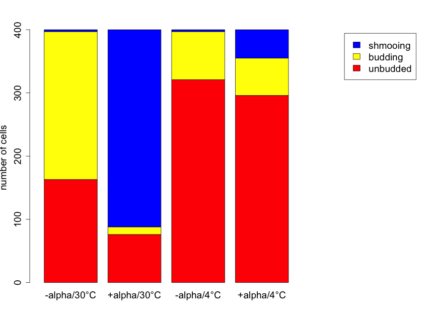
From this plot, there is the strong suggestion that yeast cell shape is related to treatment group. At 30°C the presence of alpha factor corresponds with a decrease in the number of budding and unbudded cells, and a large increase in the number of shmooing cells compared to the absence of alpha factor. The pattern at 4°C is different. Here the decrease in the number of budding and unbudded cells is much smaller — in the presence of alpha factor — and the increase in the number of shmooing cells is also more modest. There are far more unbudded cells (regardless of alpha factor) at 4°C than at 30°C. With no alpha factor the number of schmooing cells is very small, and much the same, for both temperatures but alpha factor presence results in a far greater increase in the number of shmooing cells at 30°C than at 4°C. .
The null hypothesis for this test is that the proportion of cells with each of the 3 shapes is the same for all four treatments. The alternative is that they are not all the same. One can think of the null as stating that the yeast cell shape proportions do not depend on treatment combination. Thus, this test of homogeneity assesses whether or not the patterns of proportions are homogenous (the same) across the four treatment combinations.
With two-dimensional tables such as this, the appropriate degrees of freedom can be written as (#col-1) * (#row-1). With 3 columns (shapes) and 4 rows (treatment combinations), there will be 2 * 3 = 6 df.
We now must calculate the expected values assuming that the null hypothesis is true. We note that 856 of the total of 1600 cells are unbudded. Thus, overall, 0.535 = (856/1600) is the proportion of all cells that are unbudded. According to the null, the proportion of unbudded cells is the same for each of the 4 treatment combinations. Thus, for each combination, the expected number of unbudded cells is 214 = (400 * 0.535).
Each cell is in a given row and given column. The expected value for any cell can be expressed as (row total) * (column total) / (grand total). (This is logically equivalent to the calculation shown in the previous paragraph but is often easier “mechanically”.) Thus, for the cell with the -alpha/30°C treatment and unbudded, the expected value can be written as 856 * 400 / 1600 = 214, identical to the value given above. Using this procedure, all expected values are shown in Table 6.2.3.
| Treatment combination | Expected # unbudded cells | Expected # budding cells | Expected # shmooing cells | TOTALS |
| -alpha/30°C | 214 | 95.25 | 90.75 | 400 |
| +alpha/30°C | 214 | 95.25 | 90.75 | 400 |
| -alpha/4°C | 214 | 95.25 | 90.75 | 400 |
| +alpha/4°C | 214 | 95.25 | 90.75 | 400 |
| TOTALS | 856 | 381 | 363 | 1600 |
Again, [latex]X^{2}=\sum_{all cells}\frac{(obs-exp)^2}{exp}[/latex].
Thus, [latex]X^{2}=\frac{(163-214)^2}{214}+\frac{(234-95.25)^2}{95.25}+ ... +\frac{(45-90.75)^2}{90.75}= 12.15 + 202.12+...+23.06=1210.80[/latex]
From the chi-square tables with 6df, we see that 1210.8 is far higher than the 0.01 threshold of 16.81. Thus, p-val < 0.01 (the R commands for this test are in the Appendix). From R, the p-value is less than 10-15. The evidence is extremely strong against the null hypothesis. There is strong evidence that the distributions of yeast cell shapes are not all the same (not homogenous) for the four treatment combinations. Although some further analysis is possible, a careful study of the stacked bar plots indicates where the major differences lie. The largest difference among the 4 treatment combinations is in the number of shmooing cells. For +alpha/30°C, over 3/4 of all cells are shmooing whereas the proportion is much smaller for the other three combinations. We can also see that at 4°C, the impact of alpha factor on yeast cell shape is much smaller than it is at 30°C.
The interpretation of this test could be reported in a “Results” section as follows.
The null hypothesis that the proportion of cells with each of the three shapes — unbudded, budding, and shmooing — is the same for each of the four treatment groups — -alpha/30°C, +alpha/30°C, -alpha/4°C, and +alpha/4°C — is very strongly rejected with a p-value less than 10-15. At 30°C the presence of alpha factor corresponds with a decrease in the proportion of budding and unbudded cells, and a large increase in the proportion of shmooing cells. At 4°C there is a modest increase in the proportion of shmooing cells in the presence of alpha factor with a corresponding decrease in the proportion of unbudded cells. In comparing proportions at 4°C and 30°C for cells without alpha factor, there is a substantially higher proportion of unbudded cells at 4°C (with almost no shmooing cells at either temperature). In the presence of the mating pheromone, the proportion of unbudded cells is substantially higher and the proportion of shmooing cells is substantially lower at 4°C compared with 30°C .
