Biocore Statistics Primer
Chapter 1: Basic Concepts and Design Considerations
Section 1.1: Thinking about data
Upon obtaining data from a hypothesis-based study, scientists often have the understandable desire to immediately test any underlying hypothesis they may have. In practice, this is not the best way to start. The first step should be a careful evaluation of the raw data, including one or more graphs and/or plots and a number of useful summaries. Such a step can help you to understand the main patterns, catch errors, and, with experience, provide some indication of whether there might be some difficulties with the assumptions that will underlie the statistical tests you perform.
However, before we describe useful methods for plotting and summarizing your data, it will be helpful to introduce some key ideas that will allow you to place your observed data within the larger framework of the statistical process.
Variation and Variability in Biology
Let us begin with a brief discussion of variation and variability. The terms — variation and variability — are sometimes used differently when considered in a biological context or a statistical context, although the basic underlying ideas are related.
All biological systems vary — a lot or a little. Indeed, biological evolution relies directly on the capacity of biological systems to vary. We will refer to this basic principle, the capacity or capability to vary, as biological variability (the biological ability to vary).
Biological variability is based on the natural inherent genetics of an individual organism and on how, when, and to what extent genes are expressed with expression most often modulated by environmental factors. Natural variability is a combination of both environmental and individual variability. As an example of natural, environmental variability, yeast suspended in solution would be exposed to varying oxygen levels, depending on their location in a non-shaking flask. Those at the top of the flask would receive greater oxygen exposure than those at the bottom. It is to be expected that the environment can vary from location to location, even in a system as small and isolated as a flask, test tube, or beaker.
Natural, individual variability refers to the differences among organisms, within groups of organisms, or to differences within individuals over time. For example, the amount of body fat on an individual can affect the readings of an electromyogram (EMG) signal measured at the skin’s surface. This is because a participant with a higher level of body fat will produce a less intense and more variable EMG signal than a participant with lower body fat due to the closer proximity of electrodes to muscle. An individual’s body fat content may vary over time as well.
As noted, the usages of the terms — variability and variation — can differ between biologists and statisticians. In this primer we will try to be consistent as possible in describing the concepts.
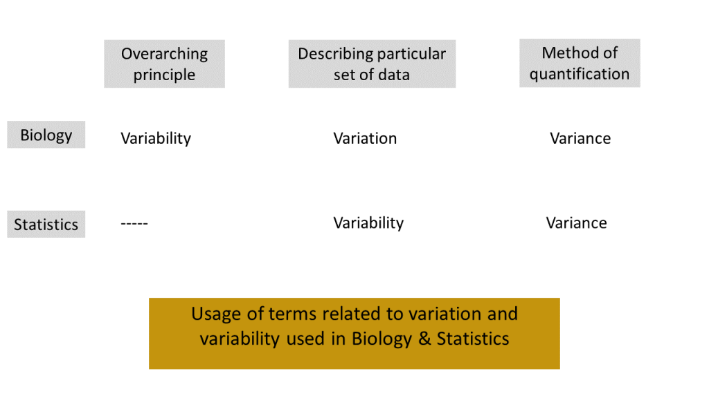
We view the notion of biological variability as an underlying principle. When we, as scientists, observe data from a biological study at a particular time point, we see that the measured values vary. As biologists, we refer to this “varying in a particular set of data” as biological variation. On the other hand a statistician would likely refer to this as statistical variability. Whether you are a biologist or a statistician, you will quantify the extent to which the numerical data vary using the notion of variance. Figure 1.1.1 illustrates the relationship among the ideas we have described. (Note: The standard deviation is the square root of variance and this is often used instead of variance. The specific definitions of (sample) variance and standard deviation will be given in the next chapter.)
For the remainder of this section, we will use the term “variation” from the viewpoint of biologists.
Experimental results must be repeatable in order to be accepted as valid. The main reason for requiring this repeatability is that there will always be variation in the data.
Consider the example comparing the heights of 10 plants from each of two species. Each time you take a sample of 10 plants from a population, your data will reveal variation. If you were to take a second sample of size 10 from the same population, you would obtain different values. In every biological study, there will always be variation. No matter how careful we are and how uniform our material may be, the data obtained from studies are never exactly repeatable.
There are many causes or sources of variation. Some of these sources are individual (e.g., genetic or organismal) variation. There is also environmental variation. Environmental variation can often influence the individual variation. There is also experimenter and/or equipment variation, which reflects the unavoidable variation introduced by human behavior during an experiment. As scientists, we do all we can to minimize variation but recognize that there will always be at least some uncontrolled variation in every study.
Laboratory experiments are usually repeated many times before they are published. Field experiments are usually repeated or are carried out at more than one site and/or at multiple times. Replication is especially important in field experiments. Natural systems vary in space and through time. Replication helps the experimenter differentiate between natural variation and changes caused by the experimental treatment under study. Experimenters are looking for patterns in the data that can be attributed to the effect of an experimental treatment by being able to separate these patterns from the variability (natural and human-induced).
Immediately below is a short video to expand on the notions of variation and variability.
Section 1.2: Populations and Samples
Scientists use data from samples (almost always fairly small), to draw conclusions about larger populations. For example, suppose you are interested in the effects of the herbicide glyphosate (also known as ®Roundup) that enters Lake Mendota via runoff from Madison city parks and from other sources. Daphnia magna is a well-known aquatic indicator species that can serve as an excellent test species for examining this question. (D. magna are freshwater, filter-feeding invertebrates that are just a few millimeters in size. The health of D. magna populations is often used as an indicator of environmental health.) You would probably wish to think of all of the D. magna in Lake Mendota at the time of your study as your population.
A population is “the set of all individuals for which you wish to draw conclusions in a particular study.”
Obviously, in Lake Mendota, it would be an impossible task to capture and examine the entire population of D. magna. Indeed, the population is not even static in that individuals die and new ones are born. A logical approach is to study a small “representative subset” of the D. magna population and then generalize your conclusions to the whole population in Lake Mendota. In other words, you need to select a sample of D. magna from the large population in Lake Mendota.
A sample is “a representative selection of a population that is examined to gain statistical information about the whole.”
Figure 1.2.1 describes the relationship between population and sample.
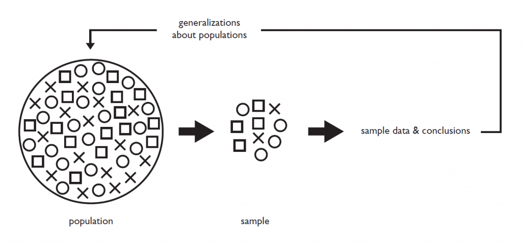
The population is made up of all the possible individuals. In Fig. 1.2.1, they are represented by the X’s, O’s, and □’s designating different groups of potential scientific interest such as different sexes, different age groups, etc. The sample is a smaller subset of individuals drawn from the population. If the sample is representative of the population, analysis can be performed on the sample data and the conclusions can then be used to make inference to the population.
It is important to define the population of interest carefully, taking into account your research question, experimental design, and resources. Here the population has been defined as the D. magna in Lake Mendota during a particular time period (usually quite short), as opposed to the entire genus of Daphnia or as opposed to all of the D. magna in Lake Mendota during a year. Obtaining a suitable, unbiased sample from a population requires care. The key element is to ensure that the sample is representative of the population.
Table 1.2.1 provides some examples of appropriately defined samples from a specified population. Keep in mind that the defined samples are by no means unique. The sample size and the method of sampling will depend on the specific goals of the study and the resources available.
| Population | Sample |
| All 250 Galapagos Finches on the island of Isabela | 45 Finches obtained from locations around the entire Isabela island via mark-recapture method |
| All of the yeast cells in a 500mL beaker | After shaking to evenly distribute the yeast in a liquid medium, 10 ml of yeast are removed as a representative sample of the beaker population |
| UW-Madison students between the ages of 18 and 22 | 150 individuals from the UW campus sampled using a random number generator from a master list of all students between the ages of 18-22. |
In some cases it makes sense to think of a population as effectively infinite. Consider the example in which you wish to compare the plant heights of two different species. Suppose that these are plants grown from seeds. Because you will never really have available an infinite number of seeds of a given species, you cannot really specify the size of the population. (If it is a common species, there are many, many sources available for obtaining seeds.) In this case it makes sense to consider the population size as effectively infinite. This will not affect the statistical procedures we describe in any way.
How many replicates should I use?
When thinking about the number of replicates to use in an experiment, scientists have to balance logistical constraints (e.g., resources, budget, time) with estimates based on statistical calculations. When feasible, scientists will often rely on statistical estimates of the variance, the most common form of quantification for biological variability. These estimates may be based on previous studies (often reported in the literature of the field) or on data from a dedicated pilot study. The number of replicates depends on both the underlying variability and the size of the effect you are trying to determine. (Greater variability will require more observations.) In some cases, if logistical constraints do not allow the number of replicates based on statistical calculations, it may be necessary to rethink the entire experiment. If your sample size is “too small”, you may be putting yourself in a position where you will be unable to reach any meaningful biological conclusions.
Biologists will rarely consider a sample with less than five independent measurements, and whenever possible will strive to obtain sample sizes that are considerably larger. In many cases 8-20 replicates may be enough; however, sometimes you will need more. Through replication, you hope to define how much of the observed variation is natural and how much is explained by your independent variable(s). An important part of experimental design is determining the experimental procedures and number of replicates necessary to reach sound scientific conclusions. (We will provide some discussion on determining sample size later in the primer.)
Types of Samples
Here, we introduce you to some well-established methods used by ecologists — and biologists in general — in designing and carrying out experiments. Ecological data often exhibit substantial variation because it is difficult or impossible to control many or most of the experimental variables in the field. Therefore, it is very important to know your system in order to anticipate variation when designing an experiment and to plan the statistical methods for analyzing data.
For example, let’s say we want to know how burning a field early in the spring influences the height of weedy Canada thistles. To run a controlled experiment, you might consider burning portions of the field while keeping other portions as non-burned (sometimes referred to as unburned). Canada thistles will grow in both the burned and non-burned portions of the field later in the season. In order to make sure the plants you measure are “representative” of all plants influenced by burning (or non-burning), you must take great care to make sure the sample is not biased. This means that it is not unduly influenced by other environmental factors such as differences in soil moisture or nutrients across the field or by how consistently the burning was done.
A key principle underlying all experimental design is random sampling. It is necessary to use a proper method for the random assignment of “treatment” (e.g. burning or non-burning) to a portion of the field. Also, if you do not measure the height of all thistles in each portion of the field (to which you randomized burning and non-burning), it is necessary to use a proper method for the random selection of plants for height measurement. If random sampling is not used and conducted properly, statistical analysis is almost always unreliable!!
As a possible design you might consider burning half of your large field but leaving the other half unburned as a control — as illustrated immediately below.
| Burn | Non-burn |
Although it may be possible to analyze data from such a design, there are very strong assumptions that must be made (even if the assignment of treatment to field half is suitably random). In reality the design illustrated above (with the large field divided into two regions) has one plot for each of the two “treatments”: burn and non-burn. You have no replication of either treatment and you cannot be sure if observed differences are due to the difference between burning and non-burning or may be due to other factors (such as soil moisture differences). You should try to avoid designs like this whenever possible.
Simple Random Sample
Consider now the case in which you divide the large field into eight plots. Suppose that you randomly assign four plots to receive the “burn” treatment and four the “non-burn” treatment. One possible assignment (out of 70 possible randomizations) might be the following:
| Non-burn | Non-burn | Burn | Non-burn |
| Burn | Non-burn | Burn | Burn |
This is the most basic type of design and is referred to as a simple random design. Unless other information is available (such as known or suspected gradients in the field) this is the default design for randomized studies. The important aspect is that the assignment is done with proper random number generation and that you do not alter the assignment that is obtained from the randomization. (Some information on how to perform such a randomization with a random number generator is given in the Appendix.)
Randomized Block Sample
Suppose that you divided your large field into 16 plots with 4 rows of 4 plots each. Suppose further that you suspect that there may be a soil moisture gradient from the upper left to lower right of the field. A simple random sample could — by chance — result in a disproportionate number of plots of one treatment in the upper left and of the other treatment in the lower right. This could lead to some possible confounding of treatment with soil moisture gradient that is undesirable. To avoid such confounding conditions, some researchers use use a systematic sample approach as depicted below.
| burn | non-burn | burn | non-burn |
| non-burn | burn | non-burn | burn |
| burn | non-burn | burn | non-burn |
| non-burn | burn | non-burn | burn |
Although systematic sampling is sometimes used — and in many cases might not cause major problems when standard methods of analysis are employed — it is not a recommended design, and most research scientists do not use it. Instead, they would use a technique known as blocking that results in a randomized block design. Using the hypothetical field drawn as above, with a possible gradient as described, we might consider a block as two adjacent plots in a row. (The adjacent plots could also be in a column.) Then, the two treatments are randomly assigned to one of the two plots within a block. A separate random process is used for each block. For example, you could toss a fair coin for proper random allocation.
| burn | non-burn | non-burn | burn |
| burn | non-burn | burn | non-burn |
| non-burn | burn | burn | non-burn |
| burn | non-burn | non-burn | burn |
Blocking restricts the randomization. (In the above case, we will always have 2 burn and 2 non-burn treatments within each row. The gain is that we have minimized the chance that a potential soil moisture (or other) gradient in the field will affect our results. Thus, we are removing some possible systematic variability due to the gradient.
Sampling methods are also important for studies in a lab setting. For an example of such a study, see Section A in the Addendum to this chapter.
Another Type of Sample: the Nested Design
There are many other sampling designs that are used in biological studies. Here we will briefly describe the nested design that occurs quite often, particularly in ecological studies.
Suppose you wish to determine the proportion of area in a large patch of prairie that is covered with a particular species of native grass. You can imagine that accurate and precise measurements will be very time consuming and that you can only take such measurements on a relatively small area. Researchers might divide the large prairie patch into “large quadrats” — say 10*10 meters squared. A random sample of n (perhaps 8) large quadrats might be chosen. Each of these large quadrats can be further subdivided into 100 “small quadrats” — each 1*1 meter squared. Then a sample of size k (perhaps 5) small quadrats can be chosen. The k*n (perhaps 40) small quadrats can then be viewed as a representative sample of the prairie patch. (Here we think of the small quadrats as “nested” within the large quadrats.) The statistical analysis of such a design requires more complex techniques and thus is beyond the scope of this primer. It is important, however, to recognize such a design so that an inappropriate method of analysis is not selected. (We provide a bit more discussion about nested designs in a later chapter.)
Section 1.3: The Process of Science
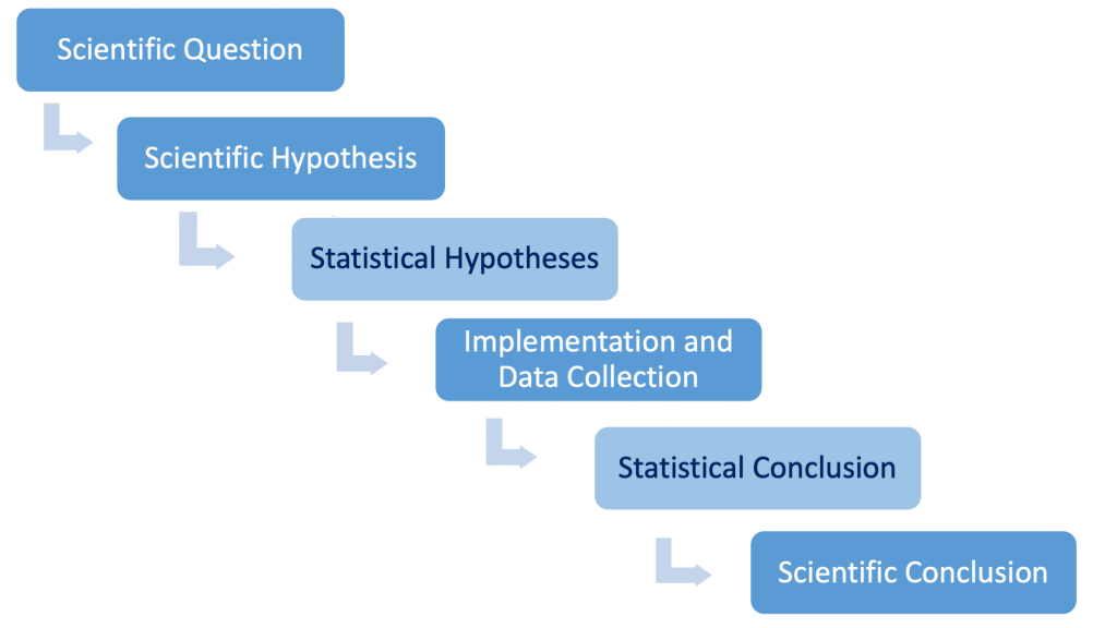
There is a very important iterative process by which scientists think about scientific or experimental hypotheses, how they can be tested, and how appropriate conclusions can be drawn using data as evidence. We will call it the Process of Science (see Fig. 1.3.1). We will focus on this logic throughout this Primer.
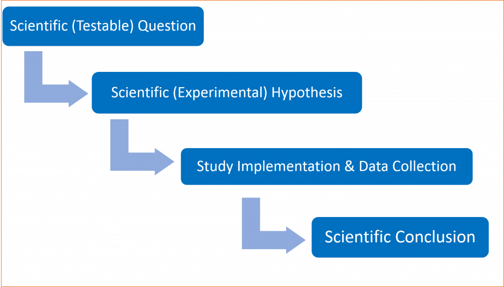
We start with a scientific or testable question. Next, we carefully phrase a scientific (experimental) hypothesis that we wish to test. Following this, we design our study and collect the data. Then, based on analysis of the data, we draw scientific conclusions. In relatively few cases we can draw the necessary scientific conclusions without recourse to statistical methods. However, for a very large number of studies conducted by biologists, statistical methods are necessary to inform valid biological conclusions.
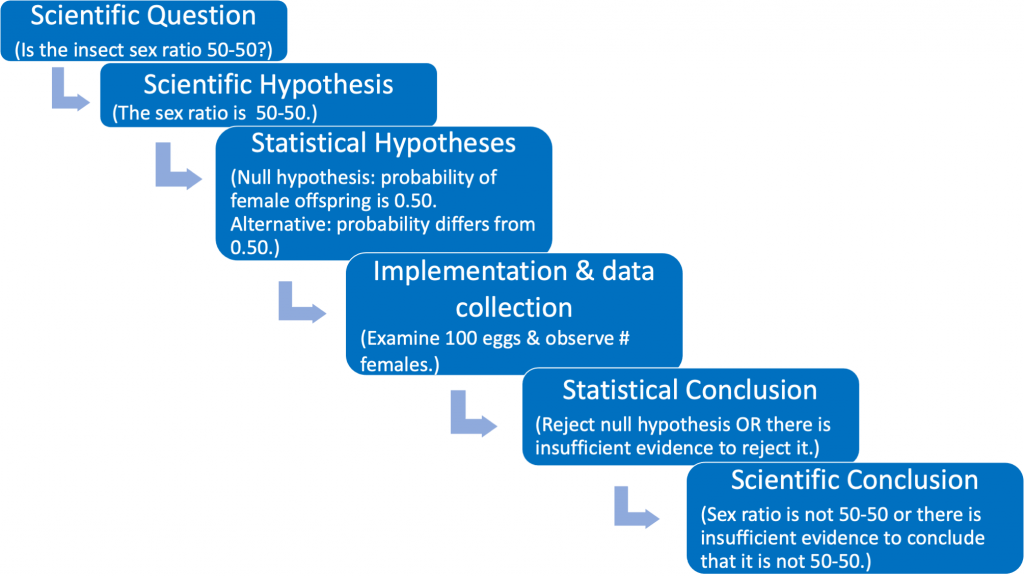
Figure 1.3.2 depicts an expanded flow chart that formally acknowledges the statistical steps. Note that scientific conclusions are informed in large part by the statistical conclusions.
We have added two boxes to the flow chart in Figure 1.3.2. The scientific hypothesis is used to phrase statistical hypotheses that explicitly define a statistical null and alternative hypothesis that will allow the inference to be conducted correctly. This step occurs with the third box. After the data have been collected, the inferential step needs to be conducted to reach a statistical conclusion. This is depicted by the fifth box. Scientists use statistical conclusions along with other considerations (e.g., their confidence in the experimental design and resulting data collected, comparison with previous published findings, etc.) to reach a logical scientific conclusion.
Let us use an example — beginning with a real scientific question — to illustrate the flow chart. Suppose we wish to examine whether or not the proportions of female and male parasitic insect offspring in a mating study are equal. We can phrase our scientific (testable) question as follows: “Is the offspring sex ratio in this mating study 50-50 or not?” (see Fig. 1.3.3).
The scientific (experimental) hypothesis can be phrased in one of two ways: [1] The sex ratio is 50-50 or [2} The sex ratio differs from 50-50 (see Fig. 1.3.4).
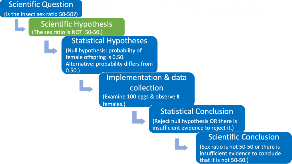
The phrasing of the scientific hypothesis is unique to each research study, and should be supported by a logical biological rationale that incorporates published literature, careful observations, and reasonable assumptions. For example, perhaps previous published studies indicate that the sex ratio is not 50-50 for the offspring of a different, but closely related, non-parasitic insect species. Based on your own pilot studies and observations, you suspect that the sex ratio for your parasitic species might also be different from 50-50, and you design an experiment to carefully document the offspring sex ratio of your parasitic species. Then you might wish to state your scientific (experimental) hypothesis using the phrasing shown in Fig. 1.3.4 (green box).
The third box in Fig. 1.3.4 states the scientific hypothesis using statistical terminology. Here it is necessary to formally articulate a (statistical) null and alternative hypothesis. The null hypothesis should be viewed as the “established” viewpoint. Sometimes it can be thought of as the viewpoint that one wishes to disprove. The null is needed so that we have a reference against which we can compare the observed results. The (statistical) alternative hypothesis can be viewed as the “challenging assertion”. In many cases the statistical alternative will be the scientific hypothesis. This occurs when the scientific hypothesis is phrased as in Fig 1.3.4 (green box). However, no matter how the scientific hypothesis is phrased the statistical null and alternative hypotheses will always be the same (see the identical third boxes in both Fig. 1.3.3 and Fig. 1.3.4).
The null hypothesis will be the “established” or “reference” viewpoint and the alternative hypothesis will always be the “challenging assertion”.
The fourth box in Fig. 1.3.4 describes the implementation of the study and the collection of data. Box #5 is the step where statistical inference takes place. Such inference is required with variable data in order to reach defensible scientific conclusions. The key concept in reaching statistical conclusions involves the the p-value, which we discuss extensively later in this primer. This step then informs the scientific conclusions illustrated by the 6th box.
Immediately below is a short video to expand on how the scientific process uses statistical thinking to inform scientific conclusions.
Section 1.4: Other Important Principles of Design
The Importance of Data from Control Groups
Suppose that you have learned that controlled burning is sometimes an effective tool for combating invasive plant species, and you want to design an experiment to test whether burning will set back the (invasive) purple loosestrife plant that is taking over your favorite wetland. You would not simply burn the wetland and see what happens because a reduction in loosestrife could be due to something other than your experimental treatment (burning). For example, it could be due to an influx of a particular insect or to the weather that year. However, if you left some of the wetland non-burned and compared the burned and non-burned portions, you could isolate the effect of burning since both portions would have been exposed to the the same additional factors (such as insects and weather). In this case the data from the non-burned portion is viewed as a control.
Medical trials also use data from control groups whenever it is possible (and ethical) to do so. Suppose a medical researcher wishes to determine whether a new drug is useful in treating a certain illness. Of the patients in the study, one portion of them (usually about half) will receive the new drug and the other portion the control (which here means no new drug). In this case the control will probably be a pill or a liquid that looks similar to the form of the new drug so that the patient does not know what s/he is receiving. (It would not be a good option for the “non-new drug” patients to receive nothing since it is well known that there is a placebo effect by which the conditions of some patients are known to improve just because they believe that they might be receiving a medication.)
Measurements: Accuracy and Precision
Since every measurement has some error, it is only an approximation of the true value. This can be thought of as another component of the variability inherent in biological data. There are two concepts related to measurement error — accuracy and precision. The accuracy of a measurement reflects how close the measurement (or the average of repeated measurements) is to the true value. The precision of a measurement indicates how well several determinations of the same quantity agree. This can also be thought of as a reflection of the repeatability of the measurements.
Consider a target that might be used in archery, with concentric rings (see Fig. 1.4.1 below). The X’s represent the locations where an arrow might hit the target. Panel [A] depicts high accuracy but low precision: the arrow hits are spread out but centered on middle of the target. Panel [B] shows high precision but low accuracy: arrow hits are close together but centered on a point away from the target’s center. Panel [C] indicates high accuracy and high precision: arrow hits are close together and centered on the target center.
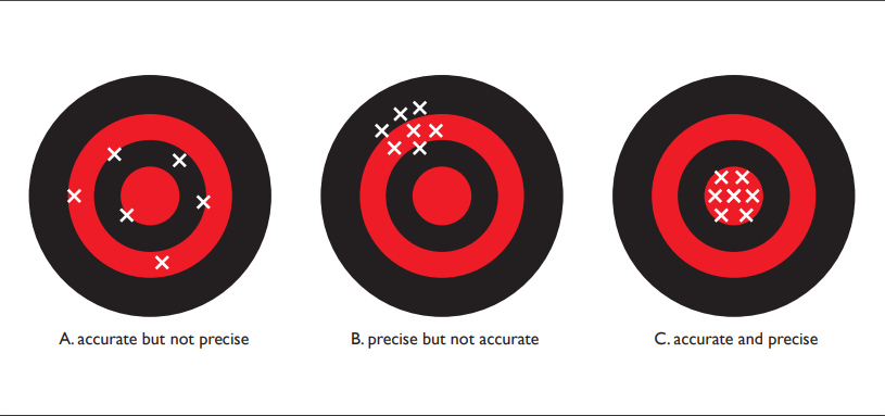
If we think in terms of data, the first case illustrates a situation where our measurements are accurate — the data are centered around the correct value — but they are not precise. In the second case, the data are precise — they are quite repeatable — but they are centered around a value that differs from the true value. (Imagine a high quality thermometer that has not been well calibrated. Repeated measurements may be very close together but they would not center around the true temperature value.) The third case shows a situation where the data are accurate and precise. In all scientific studies, it is important to understand the measurement process so that your data are as accurate and precise as possible.
There can be special issues involved with achieving precision in ecological studies. Consider an example where we compare the vegetation in wetland and prairie sites. In this type of study we divide the sites into quadrats, take a random sample of the quadrats, and take measurements (e.g. heights) of plants within each selected quadrat. Ideally we would like to examine many quadrats and take our measurements as carefully as possible. With the time, resource and budget constraints that are common in most studies, one can imagine having to make the following choice: either we can take very careful measurements on a small number of quadrats or use a quicker measurement technique but obtain data from a larger number of quadrats. The decision will depend on the specific circumstances for each study; however, in many practical cases, the quicker technique with the larger sample size is the better choice.
Statistical Independence
As we will see, all methods of statistical inference that we will use require the assumption of statistical independence. It is fair to say that, of all of the assumptions you will need to consider, this is the most important one.
The basic idea behind independence is that whatever random variation affects one data point must have no impact at all on other data points. Imagine a classroom of 20 kindergarten students. Suppose that it is known that on any given day, on average, 10% of the students will be missing due to illness. With this information, in principle (and assuming independence!!) we can calculate the probability of exactly 0 or 1 or 2 or any number of students being missing due to illness. However, the standard calculations assume that the probability that a student is missing due to illness does not depend on any of the other students. In the case of kindergarten students, it is easy to imagine that colds or some other illnesses are very contagious. Thus, knowing that one student is missing will affect probability statements about others. Thus the illness of student A and the illness of student B are NOT independent.
With quantitative data, it is often difficult to think about independence. Imagine the number of individuals of a given species of bacteria in one cubic centimeter of soil. If two samples are widely separated, it is plausible that the numbers of individuals in each sample are independent. However, if two samples are obtained in very close proximity to each other, knowing that the number of individuals is high for one sample suggests that the probability that the number is high for the other will be increased. Thus, the numbers of individuals in a cubic centimeter in the two samples would NOT be independent in this case.
The key to avoiding problems with independence in biological studies is to be careful in the conduct of your study and in the generation of your data. Attention to this issue needs to be paid at the design stage of your study. If a study has been designed that results in non-independent data, it is usually impossible to correct for this at the analysis phase. However, at the analysis phase of a study, it is necessary to carefully assess whether or not the data you are using for inference do meet the assumption.
As a specific example, consider again the controlled burning example from earlier in this chapter. Suppose you wish to make generalizations about the effectiveness of burning for control of purple loosestrife for wetlands generally in your area. You would have to locate several (typically 5 or more) different wetlands that have roughly similar density of purple loosestrife, and set up treatment (burned) and control (non-burned) areas within each. If each wetland is independent of each other (not connected or influenced by one another), then “wetland” can be considered a sampling unit and each wetland is an independent replicate. However, if one wetland is connected to another, perhaps by a small stream, then the wetlands are not completely independent of one another (perhaps they can influence each other by spread of purple loosestrife seeds in stream water). Therefore, they cannot be considered two independent replicates. The independence of replicates is of critical importance to an experimental design.
The study described in the previous paragraph can be viewed as an example of the randomized block design described earlier. In this case the blocks are the wetlands and there are two treatments per block — burned and non-burned. The number of blocks is the number of replicates. (If there is only one replicate, no statistical inference can be performed.) Later, we will provide you with some guidance in choosing the appropriate number of replicates.
Statistical Distributions: Normality
Scientists should always be familiar with the distribution of their data. We will discuss ways that data can be plotted in the next chapter. We sometimes refer to the distribution of data as the shape of the data. There is a very large number of data shapes; in Fig. 1.4.2 we refer to three of the more common ones.
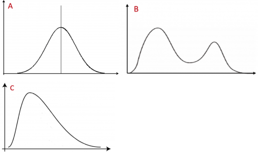
Data with a unimodal and symmetric shape have a single peak and — by definition — are symmetric. Multimodal data have multiple peaks (and may or may not be symmetric). A common type of multimodal data has two peaks and is called bimodal. Skewed data have shapes that are spread out (have a long tail) to one side and are, thus, far from symmetric. Most (but not all) such data sets have a single mode. (Also, in biology, the vast majority of skewed data sets are skewed to the right.)
Returning to our initial example on plant height, you can imagine making some kind of plot of the height values. A good plot will give an indication of the distribution of the height values. In making plots of sample data, in many, but certainly not all, cases, a majority of the observations will fall near the middle of the range of data values with fewer observations well below or well above the middle. Many statistical procedures have the underlying assumption that the data follow a symmetrical bell-shaped curve — which is a particular example of a symmetric unimodal distribution. This is described as a normal distribution (see Fig. 1.4.3).
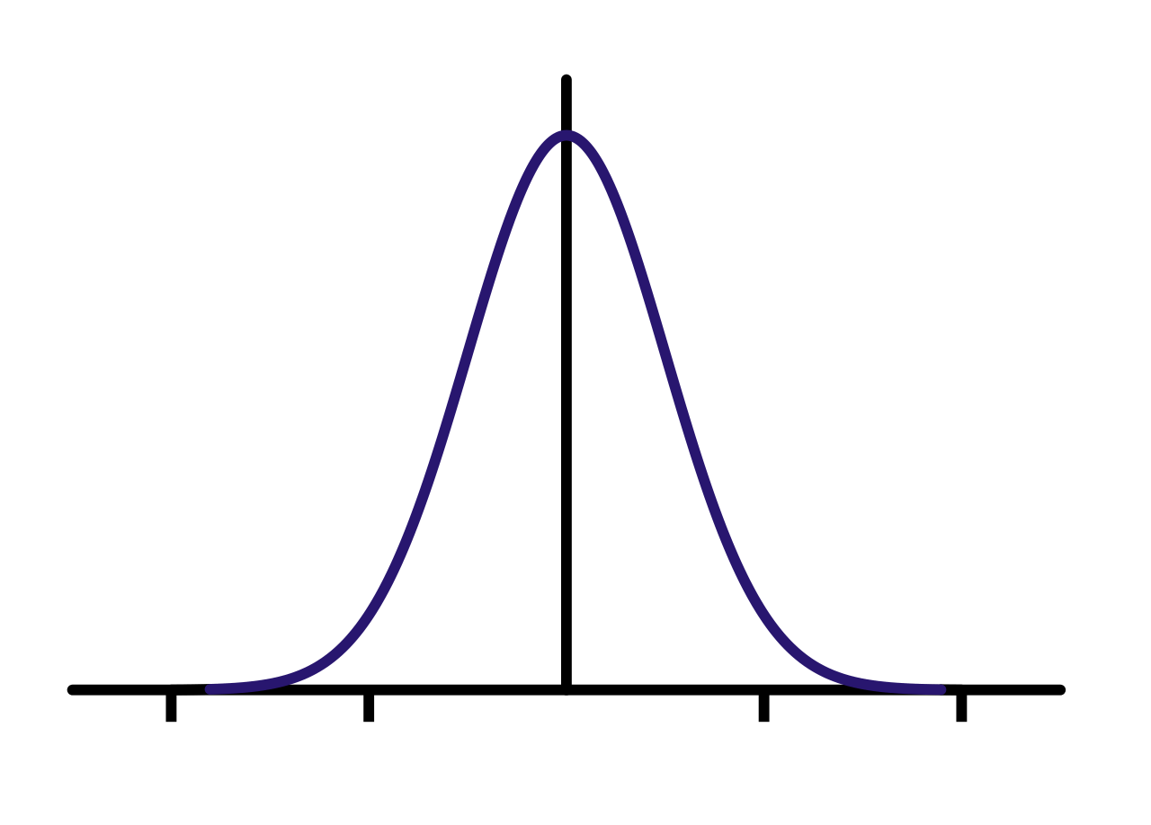
In later chapters we will discuss the role that this assumption plays in inference. For now, it is useful to recognize that the distribution of data is an important consideration for proper analysis.
Addendum to Chapter 1
Section A
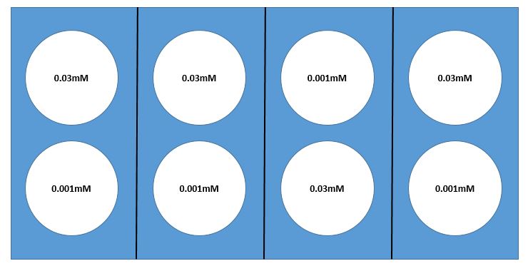
Here we present an example of a laboratory experiment where sampling issues need to be considered. Suppose you wish to determine how reaction rate of a particular enzyme is dependent on substrate concentration. You would test varying substrate concentrations, keeping enzyme concentration constant. Suppose you choose two substrate concentrations, 0.001mM and 0.03mM, with 4 replicates of each, for a total of 8 test tubes.
The assay that tests the reaction rate requires the use of a warm water bath, but we don’t know for certain that a water bath will heat the water evenly. Suppose that there is a rack with 8 test-tube holders in the water bath. If you are confident that the water temperature is quite uniform throughout the bath, it would make sense to use a simple random sampling design. However, if you are concerned about non-uniformity in the temperature — perhaps one side of the bath is warmer than the other (or maybe water near the edges is cooler than that near the center) — it would probably be best to use a random block design. Your goal should be to select blocks so that water temperature is as uniform as possible WITHIN each block and most of the expected differences are AMONG blocks. If you are concerned that one side of the bath may be warmer than the other, you might use a design with four blocks and choose your blocks as illustrated in the diagram below (Fig 1.ADD.A.1). Whatever design you select, it is always important to use appropriate randomization methods in assigning test tubes to location in the water bath. (You could “flip a fair coin” for allocation of substrate concentration within each block. Here there will be 16 [latex](= 2^{4} )[/latex] possible randomizations.)