Note: The comparison below is between this text and the current version of the text from which it was adapted.

additions / deletions

Section 3.1: Introduction to Inference
Recall the data in Table 2.2.1 representing the measured heights of 18 randomly selected lupine plants in the Biocore Prairie. How can we use such data, with corresponding plots and summary statistics, to make biological conclusions about the entire population of Biocore Prairie lupine plants? Using data from samples to draw conclusions about populations is called statistical inference.


 Statistical Inference: Using sample data to draw conclusions about populations.



After creating the appropriate plots and descriptive measures from your collected sample data — and carefully evaluating them —  you are now ready to consider some of the more formal tools of statistical inference.  In general, for any specific inference problem, there is no single "correct" tool — and often there is no single "correct" result that is obtained at the end.  There are, however, many statistical inference tools that are inappropriate and that will lead to "incorrect" conclusions from your data.  Here we intend to provide you with a solid grounding as to which statistical tools might make sense for  your own sample data.

Most statistical inference takes one of two forms: estimation (usually with confidence intervals) and hypothesis testing. There are close connections between the forms, and, in almost all cases, the results are consistent with one another.   In biology, hypothesis testing is probably the more widely used procedure. However, confidence intervals can be very helpful in some circumstances.

We make one additional distinction that is often useful.  Inference can either be “parametric” or “non-parametric”.  Parametric inference requires some assumptions about the distribution of the data (e.g., the assumption that data are normal, meaning that they follow approximately a bell-shaped curve).  Non-parametric methods make weaker or no assumptions about the distribution of the data, although other assumptions — such as the independence of the data — are required.   Virtually all commonly used methods of inference require independence.  As we will point out, the assumption that data are approximately normal is often not nearly as important as the other assumptions, even with inference methods assuming normal data.

Most inference that is performed in biology is parametric. However, in some particular situations of inference , non-parametric methods may be used. In Table 3.1.1 we provide a list of some of the more common tools for both parametric and non-parametric inference.
Table 3.1.1: Parametric and Non-parametric inference tools for hypothesis testing and estimation. Parametric inference requires assumptions about data distributions, e.g., the assumption that data are normal.



Hypothesis Testing
Estimation


Parametric
Standard procedures; t-tests, F-tests, etc.
Confidence intervals


Non-parametric
Chi-squared tests, specialized procedures; computer-intensive methods
Computer-intensive methods



Section 3.2: Confidence Intervals for Population Means
Scientists often use their sample data to estimate population values such as population means. The most useful sort of estimation allows scientists to report their level of confidence in knowing that the true population mean lies within a stated range of values. For example, this might be a statement such as, "We are 95% confident that the average resting heart rate of all swim team members lies between 50 and 62 beats per minute."

 In the previous chapter, we discussed how the standard error (SE) is used to describe the variability in using $latex \overline{y}$ (the sample mean) to estimate $latex \mu$ (the population mean).  We can provide a sharper inference statement by using the SE to compute a confidence interval (CI) for population mean $latex \mu$.

Equation 3.2.1:                    $latex \overline{y}\pm t_{n-1,\alpha/2}\times se(\overline{y})$

At first, this equation may look a bit daunting.  However, the terms can be straightforwardly described.  When the shape of the underlying data is fairly close to normal and the population standard deviation, $latex \sigma$, is unknown, we cannot directly use the normal distribution for inference.  We use something close to the normal called the t-distribution.  The t-distribution is indexed by the degrees of freedom (df).  For this application, df=n-1 where n is the sample size.

Expand to to obtain more information about the t-distribution and degrees of freedom.
Like the normal, the t-distribution is symmetrical; however, the "tails" of the distribution are a bit wider to account for the fact that we must estimate $latex \sigma$, the population standard deviation, using the sample standard deviation. The smaller the sample size, n, the more uncertain is our estimate of $latex \sigma$.

[caption id="" align="aligncenter" width="408"] Figure 3.2.1: t-distribution for various degrees of freedom ($latex df= \nu$)[/caption]

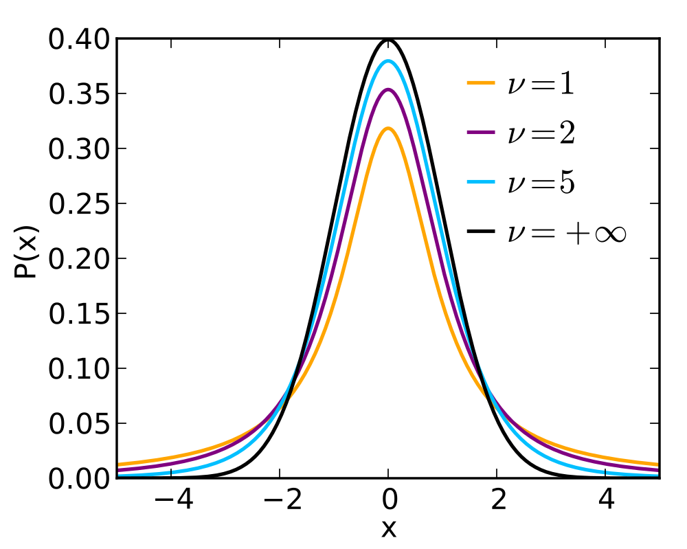
When df=$latex \infty$, the t-distribution is the same as the standard normal distribution (a normal with mean 0 and standard deviation 1) since, with an infinite sample size, the estimated standard deviation is identical to the population value. As the sample size becomes smaller, the uncertainty in the estimate of the standard deviation causes the tails of the t-distribution to become wider.

Determining the correct degrees of freedom (df) can sometimes be challenging.  Basically the df relate to the uncertainty with which the sample variance estimates the population variance.  It can be useful to think of df as "pieces of information".  We present an example that relates directly to our application of the t-distribution here.

Suppose you have a sample of 3  observations on a variable y (n=3) with values $latex y_1=7$, $latex y_2=11$, and $latex y_3=12$.  Think of this as providing 3 pieces of information about the variable.  We can see easily that the (sample) mean is 10 ($latex \overline{y}=10$).

 Recall the definition of sample variance from Chapter 2.
$latex s^2=\frac{1}{n-1}\sum_{i=1}^n(y_{i}-\overline{y})^{2}$
Let us look at the deviations $latex (y_{i}-\overline{y})$.

$latex (y_{1}-\overline{y}) = 7-10 = -3$
$latex (y_{2}-\overline{y}) = 11-10 = 1$
$latex (y_{3}-\overline{y})= 12 - 10 = 2$

Note that the sum of the deviations equals 0.  Thus, only 2 of the 3 deviations are necessary for determining $latex s^2$ since, if you know any 2 of them, the third is known since the sum is 0.  Thus, we can say that of the original 3 pieces of information in the original data, 1 piece "goes to" the sample mean and 2 pieces "go to" the sample variance.  Thus, there are 2 df for the variance and for the t-test.  (This also helps explain the use of (n-1) in the denominator for the sample variance.)

 

There are different levels of precision for specifying a CI.  Most biological scientists use a 95% CI as a standard.  However, depending on the particular circumstance, one can use 90% or 99% or any other value for the precision.  The Greek letter $latex \alpha$ in the CI equation is a proportion directly related to the desired precision.  For a 95% CI, $latex \alpha$ becomes 1-0.95=0.05.  To obtain the appropriate t-value to use, it is necessary to use specialized tables.  (We present a table in the Appendix to this primer.) These t-values can also be obtained from many computer packages including R.

The term $latex se(\overline{y})$ in equation 3.2.1 for the CI is the standard error of the mean, defined earlier.   The standard error of the mean is the most important term in determining the width of the CI. The width depends to a much smaller extent on the desired level of precision or "confidence"; e.g. 90%, 95%, or 99%.  Using 99%, for example, we can be "more confident" that the true value we are trying to estimate is within the interval; however, the interval will be wider than with a lower level of confidence.   Again, a level of confidence equal to 95% is the most commonly used level.

As noted earlier, the sample standard deviation is an estimate of the population standard deviation which is a fixed characteristic of the variable in which you are interested (e.g. plant height).  The key factor in controlling the precision in estimating the population mean is the sample size.  The larger the sample size, the narrower (more precise) the CI becomes.

For our lupine plant height data,  $latex \overline{y}=74.66667$, $latex s=15.28167$, and $latex n=18$.  (Note that we now carry more decimal places for s since we are using it as part of an intermediate calculation.)  Suppose we want a 95% CI for the true mean height of lupine plants.  Thus, $latex \alpha=0.05$.    Since $latex n=18$, we have 17 df for error.  In  our accompanying t-table, we go to the column headed by 0.05 for "two-tails".  We see that the corresponding t-value is 2.110.  Thus, plugging the values into the CI equation, we find that our CI becomes:
$latex 74.66667\pm 2.110\times 15.28167/\sqrt{18}=74.67\pm 7.60$
We could also write this as:

$latex 67.07 \lt  \mu \lt 82.27$ or, with further rounding,

$latex 67.1 \lt \mu \lt 82.3$ , where $latex \mu$ can be thought of as the population mean height of the lupine.  (Had we been interested in a 99% CI, we would have replaced the 2.110 by 2.898 (from the column headed by 0.01 for "two-tails".  This would result in the wider CI: $latex 64.2 \lt \mu \lt 85.1$).  (However, we would now be making a statement with "more confidence".)

Expand to see a short technical aside. 
You may wonder why $latex \alpha/2$ appears in Eqn 3.2.1, even though, for a 95% CI, we use the the column headed by 0.05 for "two-tails".  The standard notation used in Eqn 3.2.1 always refers to the one-tail situation.  Note that the column headed by 0.05 for "two-tails" is the same as the column headed by 0.025 for "one-tail".


Interpreting Confidence Intervals
The proper interpretation of a 95% CI is stated in terms of the researcher's confidence in the range of values containing the true population value .  For our lupine plant height data, we can say that we are "95% confident" that the true mean height lies between 67.1 and 82.3 centimeters.  It is technically not correct that there is a 95% probability that the true mean height lies between 67.1 and 82.3 cm.  The 95% refers to the procedure that is used to find the CI.  In the long run, in calculating many CI's, we can be 95% certain that the true mean lies within the CI; however, we should not say this for any individual CI.
Assumptions for One-Sample Confidence Intervals
The two key assumptions underlying this CI approach are: (a) the data are statistically independent and (b) the data follow the normal distribution. The assumption of data independence is the more important assumption.  As discussed previously, this requires a careful understanding of the study design and the way the data were collected.  If a suitably random procedure was used for selecting the 18 lupine plants (meaning that the individual plants were well separated, were representative of all the habitats where the lupine grow, etc.), then we can feel reasonably comfortable that the assumption of independence is satisfied.

With regard to the normality assumption, most normal-based inference (like the CI approach discussed here) is fairly robust to departures from normality if the data are not strongly skewed.  A  procedure  is said to be robust with respect to an assumption if the results are not overly sensitive to some departures from the assumption.  (Although our CI approach is robust to departures from normality, it is NOT robust to departures from independence.)

Sample size also plays a role in the robustness argument.  With small sample sizes, one can tolerate less skewness than with large sample sizes.  There are no agreed upon "skewness cut-offs" that one can use.   Experience is the best guideline.

If the normality assumption is not met (but the independence assumption is satisfied) there are some alternative approaches that can be used in some circumstances.  Sometimes a transformation of the data (perhaps with a square root or logarithm transformation) can be used.  In some other circumstances, it may be helpful to apply a non-parametric procedure.  We will provide an example where a transformation is helpful in a later chapter.


Assumptions for One-Sample Confidence Intervals Using Normal Theory

 	
Observations must be Independent (most important assumption!!)
 	
Data need to be (approximately) normally distributed (data must not be too skewed)


Using Confidence Intervals to Compare Population Means
Often scientists want to know whether two populations are the same or different. For example, suppose we wish to know whether burning a tallgrass prairie affects weed growth. We could gather data to address this question by treating different parts of the Biocore Prairie in two different ways.  We burn some parts and leave other parts unburned.   Then, one year later, we compare the density of thistles (bad weeds!) in the two parts by counting thistles in a large number of 0.5m2 frame quadrats that are "randomly selected". Suppose we find that the average thistle densities for burned vs. non-burned plots are different. How do we know whether the difference we observe is due to the burn treatment or simply to random variation in the samples we happened to measure?

The most appropriate formal method for answering this question is called the two-independent-sample t-test, and will be introduced in the next chapter.  However, we can utilize the single sample confidence interval approach — with accompanying graphics — to provide some approximate inferential results.

The basic idea is the following.  We can compute confidence intervals for each treatment.  If the confidence intervals DO NOT overlap, we can conclude (approximately) that the two treatment means are really different.  If the confidence intervals DO overlap, the treatment means are not different.
Representing confidence intervals graphically
We can compute confidence intervals for each treatment by multiplying the standard error by the appropriate t-value.  First, we need to consider the proper degrees of freedom (df).  For our approximate test to work, we need to consider 85% confidence intervals.  The t-tables in this Primer do not provide t-values for 85% CI's.  However, it is easy to use R to obtain such values.  Suppose we wish to find the appropriate t-value for 6 df.  With an 85% CI, we will have a probability of 0.075 in each tail.  To find the correct t-value we use 0.925 (= 1 - 0.075) in the appropriate R command.  R will return the answer of 1.65.

(If you do not have access to R, you can find an approximate value that works adequately by taking the average of the two t-values corresponding to an 80% and 90% CI.  For example, with 6 df, we obtain an approximate t-value as 1.69 (by averaging 1.440 and 1.943 from the tables,  However, if possible, it is best to use R to find the correct value.)

As an easy approximation to use in constructing CI's for the purpose described here, use the t-value according to the following sample size ranges:

for $latex n\leq6$   t=1.80

for $latex 7\leq n\leq12$   t=1.58

for $latex 13\leq n$   t=1.50

We illustrate the procedure with two sets of plausible (but made-up) data comparing the density of thistles from a burn/non-burn study as described above. We use these data to make some important points about interpretation.

Suppose that 11 quadrats are randomly selected from each of the burned and unburned parts of the prairie.  The number of thistles is recorded for each quadrat. The data for the first data set, Set A, are shown in Table 3.2.1.
Table 3.2.1: Set A example thistle density data for burned & unburned prairie plots


# Thistles in 

Burned Quadrats

# Thistles in 

Unburned Quadrats


29
24


33
13


6
3


20
37


39
8


4
16


17
30


25
17


12
11


36
6


10
22





To examine the distribution of the thistle density data for each treatment, we can quickly make a side-by-side stem-leaf plot of these data by hand (Fig. 3.2.2) or by using R Statistics software (Fig. 3.2.3).



Burned    Unburned
0| 46      | 368
1| 027     | 1367
2| 059     | 24
3| 369     | 07

Figure 3.2.2:  Side-by-side stem-leaf plot for thistle example Set A (made "by hand")
 
  Burned          Unburned  	 
    1     4| 0* |3     1        	 	 
    2     6| 0. |68    3	 	 
    4    20| 1* |13    5	 	 
    5     7| 1. |67   (2)	 	 
   (1)    0| 2* |24    4	 	 
    5    95| 2. |	 	 
    3     3| 3* |0     2	 	 
    2    96| 3. |7     1	
           | 4* | 	 
    ________________________	 	 
n: 11                 11
Figure 3.2.3:  Side by side stem-leaf plot for thistle example Set A (made using R)


The far left and far right columns in Fig. 3.2.3 are of secondary importance.

Expand for a brief explanation. 
In Fig. 3.2.3, the far right and far left columns are cumulative totals from the extremes towards the middle. For example, the "3" in the second row of the far right column indicates that there are 3 unburned quadrats with less than 10 thistles. The row with the median is marked by a number in parentheses. The (2) in the 4th row of the far right column indicates that there are 2 quadrats in the row that contains the median — the row including counts from 15 to 19.  (Note ---  the row with 0* includes values from 0 to 4 and the row with 0. contains values from 5 to 9.)


Pause and Ponder: Based on these side by side stem-leaf plots, do you see any trends in thistle density data distributions, for the Set A data? Do the distributions appear similar for the burned and unburned quadrats, or are they different?

We calculate the mean and standard deviation for each of the two groups with $latex y_{b}$ and $latex y_{u}$ representing the number of thistles for the burned and unburned quadrats respectively..

$latex \overline{y_{b}}=21.0000$, $latex s_{b}=12.2719$ .

$latex \overline{y_{u}}=17.0000$, $latex s_{u}=10.4595$ .

We see that the sample means differ by 4 but the standard deviations are quite sizable and there is substantial overlap between the two distributions.  (The plots show no basis for being concerned about possible non-normality of the data.)   We now calculate the approximate 85% confidence intervals for the two groups using the procedure described above.  Because the sample size of 11 falls between 7 and 12, we use t=1.58.

burned:  $latex 21\pm 1.58\times 12.2719/\sqrt{11}=21\pm 5.85$     $latex (15.15,26.85)$ .

unburned:  $latex 17\pm 1.58\times 10.4595/\sqrt{11}=17\pm 4.98$     $latex (12.02,21.98)$ .

Thus we can say that we are 85% confident that the true mean thistle density in burned plots lies between 15.2 and 26.9 thistles, and lies between 12.0 and 22.0 thistles in unburned plots. We see that there is substantial overlap between the two confidence intervals. Thus, the Set A data provide no  evidence that the mean thistle densities are different in burned vs. unburned parts of the prairie.

Now consider the data for the second "plausible" set of data, Set B (Table 3.2.2).
Table 3.2.2: Set B example thistle density data for burned & unburned prairie plots


# Thistles in 

Burned Quadrats

# Thistles in 

Unburned Quadrats


22
14


27
24


17
16


20
18


19
15


21
12


18
21


25
20


15
15


22
13


25
19



Fig. 3.2.4  shows the stem-leaf display for Set B data.  Note that the scale on the stem-leaf displays is different than in Fig. 3.2.2!!


burned              unburned
1|              | 234
1| 5789         | 55689
2| 0122         | 014
2| 557          | 


Figure 3.2.4:  Side-by-side stem-leaf plot for thistle example Set B (made "by hand")

The sample means and standard deviations for the thistle densities for burned and unburned plots, respectively, are:

$latex \overline{y_{b}}=21.0000$, $latex s_{b}=3.6878$ .

$latex \overline{y_{u}}=17.0000$, $latex s_{u}=3.7148$ .

The sample means are exactly the same as before but the standard deviations are substantially smaller.  The  stem-leaf plots shown in Fig. 3.2.4 suggest some real separation of the distributions.     (Again, the plots show no evidence of possible non-normality of the data.)

Let us compute the 85% confidence intervals for this situation.

burned:  $latex 21\pm 1.58\times 3.6871/\sqrt{11}=21\pm 1.76$     $latex (19.24,22.76)$ .

unburned:  $latex 17\pm 1.58\times 3.7148/\sqrt{11}=17\pm 1.77$     $latex (15.23,18.77)$ .

The two intervals do not overlap.  Thus there is solid evidence that the mean numbers of thistles per quadrat differ between the burned and unburned parts of the prairie. (We offer a brief cautionary note.  If the variances for the two groups --- the burned and unburned quadrats --- differ substantially, this interval overlap method may lead to erroneous interpretations.  This is clearly not a problem here.)


(The formal tests in the next chapter will corroborate the conclusions for both Set A and Set B. Peer-reviewed scientific research papers almost always report the results of formal tests rather than on the overlap of confidence intervals.)


Note that the only difference between Set A and Set B is the magnitude of the standard deviations.  Set B has substantially less variability.  Thus, the magnitude of the variability is a key component in drawing statistical inference.

Another key factor in comparisons like these — one not illustrated with this particular example — is the sample size.  As the sample size is increased, the denominators in the CI expressions become larger and the intervals become smaller.  Again, sample size is largely under the control of the investigator although time and cost considerations will play a large role in real-world sample size determination.

We can graphically depict this comparison of sample means with side-by-side bar charts with superimposed CIs (see Fig 3.2.5).  This can be a useful way to summarize the findings from such a comparative study.

[caption id="attachment_865" align="aligncenter" width="1024"] Fig 3.2.5. Plots of mean numbers of thistles per quadrat with error bars representing 85% confidence intervals (CI), for the burned and unburned parts of the prairie for two possible data sets [A left, B right]. For both data sets n = 11, but the standard deviations for set B data are much smaller than the Set A standard deviations.[/caption]
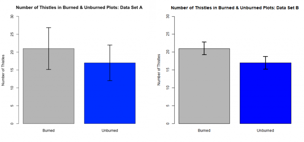
The top of each rectangle quantifies the mean number of thistles found in sample quadrats (n= 11 for each treatment group) within the burned and unburned treatment groups. The means for the burned and unburned parts are the same for each data set (21 and 17 respectively). The variances for Set B are smaller than those for Set A.  The CI bars on each rectangle represent +/- 1.58SE. With reasonable confidence, 85% in this case, the true population mean in each case lies within the end points of the CI bar. For Set A, the CI bars overlap indicating that there is too large a variance to conclude that the population means differ. The CI bars do not overlap for Set B. This suggests that the “true” means of the treatments differ.

For this thistle example, If your sample sizes were smaller, the CI bars would be wider and and there would be less evidence for a difference between the groups.  Conversely, if your sample sizes were larger, the error bars would be narrower and there would be more evidence for a difference between the groups.


 Confidence Interval (CI) bars get wider (larger) when:


 	
the sample size is decreased
 	
the sample variance is larger

 Confidence Interval (CI) bars get narrower (smaller) when:


 	
the sample size is increased
 	
the sample variance is smaller


Section 3.3: Quick Introduction to Hypothesis Testing with Qualitative (Categorical) Data --- Goodness-of-Fit Testing
In some scientific disciplines previous research findings support a specific predictive model. Scientists may wish to compare some new experimental data to what is predicted by the model. Here we briefly provide an example, the goodness-of-fit test, to show how scientists formally test their predictive model with qualitative, categorical data. (Further discussion --- using the same example --- will be provided later.)


In genetics the dihybrid cross model predicts specific phenotypic proportions for F2 generations, given key assumptions about the parental generation.  Perhaps the most common dihybrid cross example is one with two unlinked autosomal genes that affect seed characteristics, with two alleles at each locus and complete dominance in both cases. 

Imagine that we are interested in the inheritance of two qualitative pea seed characteristics, color and texture. In this case "round" is dominant over "wrinkled" and "yellow" is dominant over "green".  For data in the F2 generation, we would expect ratios of 9 - 3 - 3 - 1 in seed characteristics.  This means that for every 16 seeds, we would expect 9 to be round and yellow, 3 to be wrinkled and yellow, 3 to be round and green, and 1 to be wrinkled and green.  Suppose a study is conducted resulting in 400 seeds in the F2 generation.  The following data are observed (Table 3.3.1).
Table 3.3.1:  Observed data for the dihybrid cross study


round and yellow
 218


wrinkled and yellow
  80


round and green
  72


wrinkled and green
  30


total
400



We can use the goodness-of-fit test to determine how closely the observed data follow the expected 9 - 3 - 3 - 1 ratios.  As noted earlier, there are assumptions that underlie all statistical inference.  The assumptions for this type of goodness-of-fit test — along with additional structure — are discussed later in the primer.

If the 400 seeds perfectly followed the 9 - 3 - 3 - 1 ratios, we would expect 225 = (400 * 9/16) to be round and yellow.  Similarly, we expect 75 to be wrinkled and yellow, 75 to be round and green, and 25 to be wrinkled and green.   Table 3.3.2 shows these observed and expected values.
Table 3.3.2:  Expected data (under the null hypothesis of 9-3-3-1 ratios) for the dihybrid cross study



observed
expected


round and yellow
218
225


wrinkled and yellow
80
75


round and green
72
75


wrinkled and green
30
25



We need a procedure for determining how close (or how far apart) these two distributions are.  The appropriate procedure (often referred to as a chi-square test) is to calculate    $latex X^2=\sum_{all cells}\frac{(observed-expected)^2}{expected}$.

$latex X^2=\frac{(218-225)^2}{225}+\frac{(80-75)^2}{75}+\frac{(72-75)^2}{75}+\frac{(30-25)^2}{25}=1.671.$

If the observed counts are close to the expected, we will anticipate $latex X^2$ to be small.  The more the observed counts differ from the expected, the larger $latex X^2$ will be.  Thus, small $latex X^2$ provide evidence that the observed data follow the expected model whereas large values indicate that the data do not support the model.  There are specialized tables for judging how small or large $latex X^2$ needs to be in order to suggest that the model is not supported.  For our situation with 4 seed phenotype categories, the tabled cutoff value — that would be used by most biologists — is 7.81.  Thus, our $latex X^2$ value of 1.671 is much smaller than the cutoff and, thus, our observed data are fully consistent with the 9 - 3 - 3 - 1 model.  (If you had a test using data with only two categories, the tabled cutoff value would be 3.84.)  We will provide more complete chi-square tables — and more information about the chi-square distribution — later in the primer.
Section 3.4: Hypothesis Testing with Quantitative Data
Earlier in this chapter we used confidence intervals as a way to compare the thistle densities in burned and unburned parts of the prairie.  We were actually using the confidence intervals as a proxy for a hypothesis test.  There is a particular structure to the way in which hypothesis tests are carried out.  We introduce this logic here.
Parametric Inference Assuming Normal Data vs. Non-Parametric Inference

 If scientific data are continuous (or close to it) then inference based on an underlying distribution can often be used.  For most scientific investigations resulting in continuous sample data sets,  far and away the most commonly used underlying distribution will be the normal.  If your sample size is fairly small, it is important that the distribution of the data is not too far from normal.  If the sample size is large, you can tolerate more discrepancies from normal; however, it is important that your data are not strongly skewed to the right (i.e., when there are some data points that have much higher values than the majority of the data). 

Some scientific studies result in very small sample sizes.   Sometimes it can be very difficult to assess whether or not the assumption of approximate normality is  valid. Here is an example of data that are skewed (to the right).

2 | 348
3 | 6
4 |
5 |
6 |
7 | 5

Figure 3.4.2:  Possible skewed data set resulting from a very small sample size

If a small data set is not highly skewed like the example in Fig. 3.4.2, the use of methods based on normality can be applied with minimal risk.  This is known as the robustness of the methods of inference based on the normal assumption.

Other techniques will be needed for highly skewed data.   We will briefly discuss, later in this primer, one commonly used approach that is sometimes helpful for performing inference when the data are not (at least approximately) distributed as a normal.  This entails transforming the data.  If a transformation of the data — perhaps using a square root or log transformation — modifies the shape to appear approximately normal, then parametric methods can be applied to the transformed data and appropriate inference can be drawn.  Taking a log or square root transformation of the data in Fig 3.4.2 will result in a distribution that is far less skewed. Researchers must be particularly careful, however, to make appropriate biological conclusions from transformed data sets.

There is a field of statistics called non-parametric inference that can be applied in some circumstances.  The methods most commonly used are beyond the scope of this primer.  There are some fairly straight-forward methods that are occasionally applied.  These were quite common before it was understood how robust the methods based on normality are in practice.  (These include the Mann-Whitney test and the Wilcoxon signed-rank test.  You might encounter these is some older literature but their use is decreasing.)
Hypothesis Testing with a Single Sample (using normal theory)
Although many experimental designs result in the comparison of two (or more) groups, there are some cases where conducting a test with a single sample may be useful. We will refer to the methodology developed here as hypothesis testing.  Many statisticians prefer the term significance testing but we will use hypothesis testing.

Let us return to the lupine prairie plant example.  Suppose you were told that there was a reason to expect that the true mean height of lupine plant in a prairie of interest is 65 cm.  This "target height" could come from experience and/or literature describing other prairies.  You wish to test this claim.

It is helpful at this point to introduce a bit of statistical notation.  Let $latex Y$ be the height of an individual lupine plant.  Since we will be using normal theory, we can write:

$latex Y\sim N(\mu,\sigma^2)$.

This reads that $latex Y$ is distributed as a normal distribution with population mean $latex \mu$ and population variance $latex \sigma^2$.  Here, $latex \mu$ and  $latex \sigma^2$ are the population counterparts to the sample mean $latex \overline{y}$ and sample variance $latex s^2$.  (It is certainly correct to think that $latex \overline{y}$ estimates $latex \mu$ and $latex s^2$ estimates $latex \sigma^2$.)
Stating the statistical hypotheses

In Chapter 1 we described the iterative Scientific Process which includes the important step of stating the statistical hypotheses.  With $latex \mu$ as the mean height, we state that our null hypothesis is that the true mean height is 65 cm.  There are three possible alternative hypotheses that could be chosen.

 	
Alternative Hypothesis 1:   Either $latex \mu$ < 65 or $latex \mu$ > 65   (two-sided alternative)
 	
Alternative Hypothesis 2:  $latex \mu$ < 65   (one-sided alternative)
 	
Alternative Hypothesis 3:   $latex \mu$ > 65   (one-sided alternative)

In almost all cases, the default alternative hypothesis is the first one --- the two-sided alternative.  However, it is possible that, in some specific circumstances, you might consider one of the one-sided alternatives.  For example, you might be in the nursery business and wish to assure your customers that the mean height of the lupines you sell is at least 65 cm.  If the mean height is larger, there is no problem.  If the mean height is less than 65 cm, then you would not be in a position to sell your lupines.  In this case you might wish to consider Alternative Hypothesis 2.  It is important that the sidedness of the alternative be selected before any study is conducted, based on prior scientific knowledge obtained from previously published, peer-reviewed findings from similar research studies, if at all possible. Allowing your own observed data to influence the sidedness is bad science and in some cases even unethical.  We will consider an example for which a one-sided alternative is clearly appropriate a bit later.

You might argue that it is almost certain that the mean height cannot be exactly 65 cm.  That is almost certainly true.  The question answered by hypothesis testing is the following: Do the sample data provide sufficiently strong evidence against the null hypothesis (that the true population mean is 65 cm) to cause us to state that the null is false? (Recall our sample lupine plant height data, where sample mean  cm, , and .) 


Hypothesis testing answers this question: Do the sample data provide sufficiently strong evidence against the null hypothesis?


For our lupine prairie plant height data, we can symbolically state the null (Ho) and alternative hypotheses (HA) as given below.  We strongly recommend that you  take the time to formally write your hypotheses in this way before collecting sample data!!

$latex H_{0}:\mu=65$
$latex H_{A}:\mu\neq65$
Performing the one-sample t-test

Using normal theory — and a distributional approach similar to that we used for creating confidence intervals — the desired test of our hypothesis is the one-sample t-test (or single-sample test).   We calculate the test-statistic "T".

$latex T=\frac{\overline{y}-\mu}{s/\sqrt{n}}$

Here, $latex \overline{y}$ is the observed sample mean and $latex \mu$ is the value for the population mean if the null hypothesis is true.  The denominator is our old friend, the sample standard error.  Basically, we are comparing the difference between $latex \overline{y}$ and $latex \mu$ with the standard error.  If T is large in magnitude, there is evidence that the sample mean $latex \overline{y}$ is not close to the population mean $latex \mu$. (Note that smaller standard error values --- which result either from smaller standard deviation values or larger sample sizes --- also increase the magnitude of T.)

With the summary statistics for the sample lupine data given above, we can calculate our T.

$latex T=\frac{74.66667-65}{15.28167/\sqrt{18}}=2.684$

Since the alternative hypothesis is two-sided, we argue that an observed value of $latex \overline{y}$ of 55.33333 cm is equally distant from the null hypothesis value of 65 cm as is 74.66667 cm.  A $latex \overline{y}$ value of 55.33333 results in $latex T=-2.684$.

To quantify how "discordant" our sample mean height value of 74.7 cm is from the expected value of 65 cm, based on this value of T, we calculate a "p-value"  which, for this example, is the probability of obtaining a sample mean as far away from the population mean as we observed or larger.  This can be thought of as quantifying how rare it is to observe a difference between the sample and hypothesized population means this large or larger. This quantification requires use of the t-distribution.   Again, we recognize that the alternative is two-sided.  We define

$latex p-val=Prob(t_{df}(2-tail-proportion)\geq T)$ .

For the lupine data,

$latex p-val=Prob(t_{17},(2-tail-proportion)\geq 2.684)$ .

The "2-tail proportion" takes into account that we are calculating the probability that $latex T$ is either as large or larger than 2.648 or as small or smaller than -2.648.  (The $latex t$-distribution is symmetric about 0.)

We now look at our t-table focusing on the row with 17 df.  We see that the T-value of 2.684 falls between the "two-tails" columns headed by 0.02 and 0.01.  Thus, we can write the result as

$latex 0.01\leq p-val\leq0.02$ .

Our p-value is between 0.01 and 0.02.  (Using a program such as R, we can compute this exactly.  Here, p-val= 0.017.)    Thus, if the null hypothesis that the true mean lupine height is equal to 65 cm is true, we have between a 1% and 2% probability of obtaining a sample mean as far (or further) away from 65 than we observed.  Many biological researchers use 5% as a threshold.  If the calculated p-value is less that 5%, as it is in this example, then we can conclude that the null hypothesis is false and we believe the alternative to be true. In other words, our sample data (with mean lupine height = 74.7 cm and s = 15.3) do NOT support the null hypothesis that the mean population lupine plant height is 65 cm.

If the p-value is greater than 5%, then we cannot reject the null.  In that case the evidence is just not strong enough to say that the null is false.  (We provide additional interpretation of the p-value later in this chapter.)

Recall from our 95% confidence interval calculation for the lupine data, $latex 67.1 \lt \mu \lt 82.3$.  We notice that the value of 65 cm is not contained in the confidence interval.  If we reject the hypothesized value of $latex \mu$ at 5%, then a 95% CI will not contain the hypothesized $latex \mu$.  Thus, the inferences from each of the CI and one-sample t-test approaches are consistent.  (Such consistency would be true for any other two-tail proportion value such as a 90% CI and a 10% test threshold.)
Assumptions for One-Sample Hypothesis Tests Using Normal Theory
We note that the assumptions for this t-test are identical to those for the CI.  We require the observations to be statistically independent and for the distribution of the data to be approximately normal.  The same comments on robustness with the CI hold here as well.
 Observations must be Independent (most important assumption)!!
 Data need to be (approximately) normally distributed (data must not be too skewed).
The Single Sample t-test with a one-sided alternative
As noted earlier, in some single sample testing situations the alternative can be “one-sided”.   An example for which this might make sense is in testing a limit on pollution levels.   Suppose that the limit for some toxic chemical in the wastewater from some industrial plant is 5 parts per million (ppm).  Here, the null will only be rejected if the observed mean is greater than 5 ppm.

Ho : $latex \mu$ =  5 ppm
HA : $latex \mu$ > 5 ppm

(Sometimes the null is written Ho : $latex \mu\leq5$ .)

As an example of how a conclusion can be reached in such a circumstance suppose that a random sample of 10 measurements were taken on the toxic chemical concentration and the T "test-statistic" was calculated and had a value of 2.02.  We now enter the t-tables using the values for "one-tail".  With 9 df (since n=10), we find $latex 0.025\leq p-val\leq0.05$ .  (The exact p-value can be calculated with R). Because the calculated p-value is less than 0.05, we can conclude that the null hypothesis is false and we believe the alternative to be true. In other words, the sample data indicate that the population mean value for this chemical is greater than the wastewater limit of 5 ppm.

The overwhelming majority of statistical tests are performed with two-sided alternative hypotheses.  A one-sided alternative should be used only in in circumstances like those suggested with the "pollution limit" example.
Section 3.5: Interpretation of Statistical Results from Hypothesis Testing
The p-value
Scientists often propose hypotheses and then do experiments to see whether the world functions in a way consistent with their hypotheses.  We described this "Process of Science" in an earlier chapter.   While it is not possible for experimental data to prove that a particular model or hypothesis is correct or false, we can determine whether or not results differ significantly from those predicted by the null hypothesis.   The question then is: what is meant by "differ significantly"?  How far from the predicted or expected values can the data be before it is necessary to reject our statistical null hypothesis?  Chance can cause results to differ from expectations, particularly when the sample size is small.

The p-value is a particularly important summary indicator for hypothesis testing with biological data.  Think of the p-value as a measure of “rareness” of the observed sample data --- given the hypotheses.


If the null hypothesis is true (and taking the alternative hypothesis into account), the p-value indicates the probability of obtaining data as extreme or more extreme than what you observed in your sample.


As an example, suppose that you calculate a p-value of 0.03.

This DOES NOT mean:  The probability that the null hypothesis  is true is 0.03 --- or 3%.

What it DOES mean:   If the null hypothesis is true, there is only a 3% probability of seeing data as extreme or more extreme than we observed in our sample, with respect to what was expected under the null hypothesis, taking the alternative into account.

 	


 	
If sample data are close to what is expected under the null hypothesis --- then p-value is large and the null is supported.
 	
If sample data are far from what is expected under the null hypothesis --- then p-value is small and the null is rejected.





Here is a useful way of thinking about p-values:

 	
"large" p-value —> data support null hypothesis
 	
"small" p-value —> data provide evidence against null hypothesis


In order to make a decision to either reject or not reject the null hypothesis, we compare our p-value to our chosen threshold value.  Many biological researchers use 5% as a threshold.  However, there is no absolute scientific rule that can tell us what the best threshold value should be.  To a large extent it is based on conventions within each scientific discipline.  Even these conventions must take into account practical considerations such as sample size and the use that will be made of the test results.

Regardless of conventions that might focus on specific threshold values, researchers should ALWAYS REPORT THE P-VALUE in addition to providing a reject/not reject decision about the null hypothesis.


ALWAYS REPORT THE P-VALUE


In practice it is very useful to think about where p-values fall within a continuum of evidence for or against the null hypothesis (see Fig. 3.5.1).  This kind of approach is used by many statistical practitioners.


[caption id="attachment_49" align="aligncenter" width="1024"] Figure 3.5.1:  The p-value continuum providing evidence for or again the null hypothesis.[/caption]

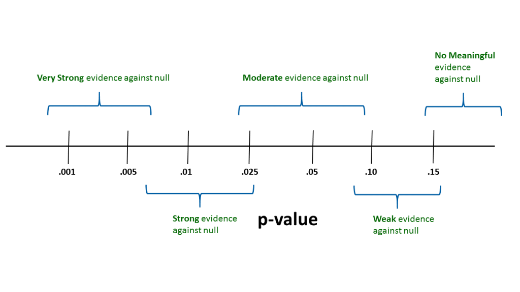
Thus, with a p-value above about 0.15, we could conclude that there is no real evidence in the sample data to cause a researcher to question the null hypothesis.  When the p-value is between say --- 0.07 and 0.16 --- we could state that there is some weak evidence against the null.  Similarly, with p-values between say --- 0.02 and 0.08 --- we might conclude that there is moderate evidence against the null.  This logic can be continued to smaller p-values.

Suppose a scientist uses a threshold of, say, 5%.  The scientist would reach a different conclusion with a p-value of 0.048 than s/he would with a p-value of 0.052.  The difference in the sample data that could result in such a small difference in p-value will be very small.  Thus, just to state that a result is or is not significant at 5% does not properly convey the scientific result.  Thus, reference to the continuum is strongly encouraged.

Immediately below is a short video focusing on p-values that includes some discussion of how investigators might formulate their statistical alternative hypotheses.

 

https://mediaspace.wisc.edu/id/0_jw3h4c2u?&playerId=25717641

 
Making errors in testing
We must recognize that we can make errors.  In some circumstances, our sample data could lead us to reject a null hypothesis when the null really is true OR they could lead us to fail to reject it if the null really is false.  The choice of the p-value threshold will depend in part on the potential costs of making an error.  For most biological studies, experience has suggested that a 5% threshold works well in most situations.  Thus, this is a reasonable value to use absent strong arguments against it.

If a null hypothesis is rejected at 5%, it is common for scientists to describe such a finding by stating  "the results are "statistically significant" at 5%.  (A similar statement can be made for any threshold value.)  Similarly, if a null hypothesis is not rejected at some level, we could say that the results are "not statistically significant" at that level.  It is important to realize that the term "statistically significant" has this very precise interpretation.  Sometimes, the finding is reported as the results are "significant".  However, this is imprecise as the term "significant" (by itself) carries a broad range of meanings.  Here it is good to be precise in your use of terminology (e.g., "The difference between the experimental treatment mean and the control group mean is statistically significant.")

It is also important to be precise when reporting p-values.  As noted, the decision as to whether or not a hypothesis is rejected depends on the threshold value chosen.  Suppose you choose a 5% threshold and report your findings by stating "we reject the null hypothesis at 5%".  This statement alone indicates that the p-value could be anything less than 0.05.  If another scientist believes that a 1% threshold is more appropriate, s/he would not know whether the null could be rejected.  Thus, it is always best practice to report the p-value so that your readers can make their own decisions about your results!!


Using Precise Language in Statistical Conclusions:

 	
Imprecise: "The results are significant at 5%."
 	
Precise: "We reject the null hypothesis that the lupine plant heights are the same at 5% with a p-value of 0.0194." 


Statistical Significance vs. Biological Significance
Statistical analysis is all about evaluating a degree of certainty: in your experimental design, in your data, and in your conclusions.  Whatever statistical procedure you apply to your data, always be mindful that the results of your analyses simply tell you whether your treatment produced a result that is statistically significant or not.  Statistics DO NOT PROVE anything—statistical methods just provide us with a measure of certainty in evaluating our results.

It is a different question to determine whether the differences you observe are biologically meaningful. This is a scientific rather than a statistical issue.  For example, let us say that you were able to increase the sample size in the thistle example to 500 quadrats for both the burned and unburned treatments in a prairie . Suppose you find that the mean numbers of thistles (in a quadrat) are 18.8 and 19.2 respectively for the burned and unburned treatments. Suppose, further, that a hypothesis test that the thistle densities are the same in the burned and unburned quadrats results in rejection of the null (say) at 5%.

You need to ask if the difference between 18.8 and 19.2 thistles per quadrat is biologically meaningful.  You may very well conclude that this difference is so small that it is of no real scientific importance.  In this case your results could be considered statistically significant but NOT biologically meaningful.

It is also possible to find results that are not statistically significant but could be considered biologically meaningful.  However, in such a case you will need to conclude that you cannot be certain that the differences you found in your sample data are "real" and, thus, beyond those that could be expected by chance.  If you wish to reach a more definitive finding, you will need to perform further studies, quite possibly with larger sample sizes.


Statistics do not prove anything.

Statistics provide us with a quantitative framework for accepting or rejecting null hypotheses.

It is your job as a scientist to determine whether the differences, trends, or patterns you observe are biologically meaningful.

If observed differences, trends, or patterns would be biologically meaningful but are not statistically significant, you must acknowledge that the results could have been obtained by chance and cannot allow a conclusion that the null hypothesis is false.


The Connection Between Biological and Statistical Thinking in Hypothesis Testing
Let us again refer to the "process of science" that underlies how almost all scientists view the testing scientific hypotheses.   In Fig. 3.5.2 we reproduce a flow chart describing the process. 

[caption id="attachment_866" align="aligncenter" width="1024"] Figure 3.5.2:  Flow chart for the Scientific Process that includes the relationship between statistical and scientific components of testing hypotheses.[/caption]

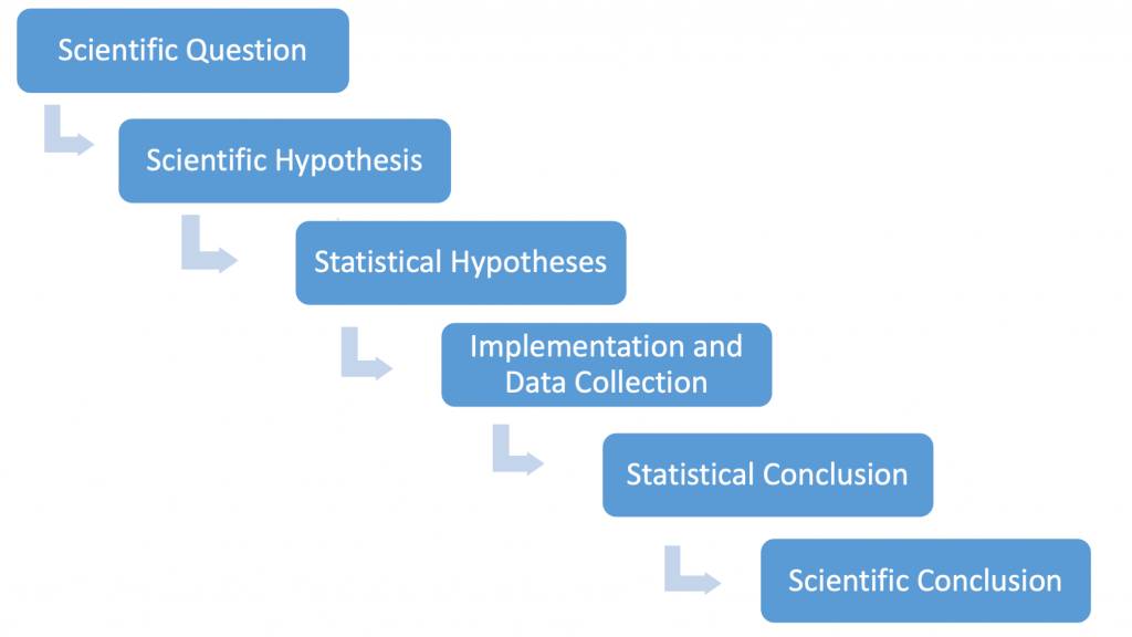
For the one-sample lupine example, a biological researcher might very well state their (scientific) hypothesis as follows: "We predict that the true mean lupine length differs from 65 cm."  Given the logic of statistical testing — that strong evidence is needed to reject a (statistical) null hypothesis — the statistical hypotheses are phrased as $latex H_{0}:\mu=65$ and $latex H_{A}:\mu\neq65$.  It is the inference step that leads to the statistical conclusions.  As noted, the p-value plays the key role here.  Here, p-value=0.016 and we are led to reject the null hypothesis at the 5% level.  The biological researcher now knows that the mean observed height of 74.7 cm is statistically significantly different from 65 cm at the 5% level.  It is now up to her/him to decide if this difference is biologically meaningful.  (This will almost certainly depend on the biological context in which the study was conducted.)

Immediately below is a short video describing the relationship between statistical and biological significance  with some comments on the proper way that results should be reported.

 

https://mediaspace.wisc.edu/id/0_swtf0tnu?&playerId=25717641