
Biocore Statistics Primer
Chapter 4: Statistical Inference — Comparing Two Groups
We are now in a position to develop "formal" hypothesis tests for comparing two samples. First, we focus on some key design issues. Then we develop procedures appropriate for quantitative variables followed by a discussion of comparisons for categorical variables later in this chapter.
Section 4.1: Design Considerations for the Comparison of Two Samples
It is very common in the biological sciences to compare two groups or "treatments". For the purposes of this discussion of design issues, let us focus on the comparison of means. (Similar design considerations are appropriate for other comparisons, including those with categorical data.) There are two distinct designs used in studies that compare the means of two groups. At the outset of any study with two groups, it is extremely important to assess which design is appropriate for any given study. In some cases it is possible to address a particular scientific question with either of the two designs. We begin by providing an example of such a situation.
Suppose that you wish to assess whether or not the mean heart rate of 18 to 23 year-old students after 5 minutes of stair-stepping is the same as after 5 minutes of rest. Here are two possible designs for such a study.
1. Independent two-sample design
You wish to compare the heart rates of a group of students who exercise vigorously with a control (resting) group. You randomly select two groups of 18 to 23 year-old students with, say, 11 in each group. All students will rest for 15 minutes (this rest time will help most people reach a more accurate physiological resting heart rate). The exercise group will engage in stair-stepping for 5 minutes and you will then measure their heart rates. The resting group will rest for an additional 5 minutes and you will then measure their heart rates.
- In this case there is no direct relationship between an observation on one treatment (stair-stepping) and an observation on the second (resting). There are different individuals in each group and the observations on each treatment are independent of each other.
You randomly select one group of 18-23 year-old students (say, with a group size of 11). You have them rest for 15 minutes and then measure their heart rates. Then you have the students engage in stair-stepping for 5 minutes followed by measuring their heart rates again.
- Here the data are obtained after resting and then after stair-stepping on the same individual. The key ingredient is that there is a direct relationship between an observation on one treatment (after rest) and an observation on the other treatment (after stair-stepping). (Note that the paired design can be a bit more general than this example. The key is always that there is a direct relationship between an observation on one treatment and an observation on the other treatment.)
For this heart rate example, most scientists would choose the paired design to try to minimize the effect of the natural differences in heart rates among 18-23 year-old students. However, both designs are possible. In most situations, the particular context of the study will indicate which design choice is the right one. Sometimes only one design is possible.
In analyzing observed data, it is key to determine the design corresponding to your data before conducting your statistical analysis.
To further illustrate the difference between the two designs, we present plots illustrating (possible) results for studies using the two designs.
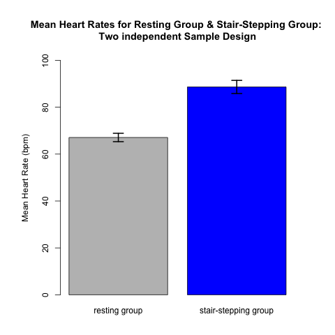
An appropriate way for providing a useful visual presentation for data from a two independent sample design is to use a plot like Fig 4.1.1. The data come from 22 subjects --- 11 in each of the two treatment groups. Each of the 22 subjects contributes only one data value: either a resting heart rate OR a post-stair stepping heart rate. Each contributes to the mean (and standard error) in only one of the two treatment groups. There is NO relationship between a data point in one group and a data point in the other. Thus, these represent independent samples. The height of each rectangle is the mean of the 11 values in that treatment group. The formal analysis, presented in the next section, will compare the means of the two groups taking the variability and sample size of each group into account.
(Note that we include error bars on these plots. Error bars should always be included on plots like these!! This allows the reader to gain an awareness of the precision in our estimates of the means, based on the underlying variability in the data and the sample sizes.)
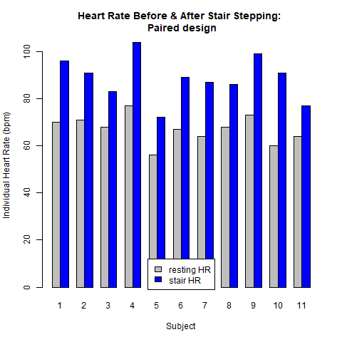
The next two plots result from the paired design. Here it is essential to account for the direct relationship between the two observations within each pair (individual student). Figure 4.1.2 demonstrates this relationship. In this design there are only 11 subjects. Each subject contributes two data values: a resting heart rate and a post-stair stepping heart rate. Analysis of the raw data shown in Fig. 4.1.2 reveals that: [1.] each subject's heart rate increased after stair stepping, relative to their resting heart rate; and [2.] the magnitude of this heart rate increase was not the same for each subject. For example, the heart rate for subject #4 increased by ~24 beats/min while subject #11 only experienced an increase of ~10 beats/min. Stated another way, there is variability in the way each person's heart rate responded to the increased demand for blood flow brought on by the stair stepping exercise.
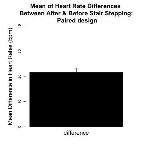
The analytical framework for the paired design is presented later in this chapter. We will see that the procedure reduces to one-sample inference on the pairwise differences between the two observations on each individual. For the example data shown in Fig. 4.1.2, the paired two-sample design allows scientists to examine whether the mean increase in heart rate across all 11 subjects was significant. Figure 4.1.3 can be thought of as an analog of Figure 4.1.1 appropriate for the paired design because it provides a visual representation of this mean increase in heart rate (~21 beats/min), for all 11 subjects.
We note that the thistle plant study described in the previous chapter is also an example of the independent two-sample design. The key factor in the thistle plant study is that the prairie quadrats for each treatment were randomly selected. There was no direct relationship between a quadrat for the burned treatment and one for an unburned treatment.
However, a similar study could have been conducted as a paired design. Suppose that a number of different areas within the prairie were chosen and that each area was then divided into two sub-areas. One sub-area was randomly selected to be burned and the other was left unburned. One quadrat was established within each sub-area and the thistles in each were counted and recorded. Now there is a direct relationship between a specific observation on one treatment (# of thistles in an unburned sub-area quadrat section) and a specific observation on the other (# of thistles in burned sub-area quadrat of the same prairie section). The proper analysis would be paired.
Section 4.2: The Two Independent Sample t-test (using normal theory)
Let us start with the independent two-sample case. We develop a formal test for this situation. We expand on the ideas and notation we used in the section on one-sample testing in the previous chapter. We will develop them using the thistle example also from the previous chapter.
Before embarking on the formal development of the test, recall the logic connecting biology and statistics in hypothesis testing:
Our scientific question for the thistle example asks whether prairie burning affects weed growth. The scientific hypothesis can be stated as follows: we predict that burning areas within the prairie will change thistle density as compared to unburned prairie areas. The statistical hypotheses (phrased as a null and alternative hypothesis) will be that the mean thistle densities will be the same (null) or they will be different (alternative). Ultimately, our scientific conclusion is informed by a statistical conclusion based on data we collect.
The proper conduct of a formal test requires a number of steps. Experienced scientific and statistical practitioners always go through these steps so that they can arrive at a defensible inferential result.
We will illustrate these steps using the thistle example discussed in the previous chapter. In that chapter we used these data to illustrate confidence intervals. Here we examine the same data using the tools of hypothesis testing.
Step 1: State formal statistical hypotheses
The first step step is to write formal statistical hypotheses using proper notation. Indeed, this could have (and probably should have) been done prior to conducting the study. In any case it is a necessary step before formal analyses are performed.
Let [latex]Y_{1}[/latex] be the number of thistles on a burned quadrat.
Let [latex]Y_{2}[/latex] be the number of thistles on an unburned quadrat.
Note that you could label either treatment with 1 or 2. The important thing is to be consistent.
Then we can write, [latex]Y_{1}\sim N(\mu_{1},\sigma_1^2)[/latex] and [latex]Y_{2}\sim N(\mu_{2},\sigma_2^2)[/latex].
It is useful to formally state the underlying (statistical) hypotheses for your test. Using notation similar to that introduced earlier, with [latex]\mu[/latex] representing a population mean, there are now population means for each of the two groups: [latex]\mu[/latex]1 and [latex]\mu[/latex]2. The null hypothesis (Ho) is almost always that the two population means are equal. Here, the null hypothesis is that the population means of the burned and unburned quadrats are the same.
We formally state the null hypothesis as:
Ho : [latex]\mu[/latex]1 = [latex]\mu[/latex]2
The standard alternative hypothesis (HA) is written:
HA : [latex]\mu[/latex]1 ≠ [latex]\mu[/latex]2
The alternative hypothesis states that the two means differ in either direction. Most of the experimental hypotheses that scientists pose are alternative hypotheses. For example, you might predict that there indeed is a difference between the population mean of some control group and the population mean of your experimental treatment group. However, statistical inference of this type requires that the null be stated as equality. Thus, sufficient evidence is needed in order to reject the null and consider the alternative as valid.
As noted in the previous chapter, it is possible for an alternative to be one-sided. However, this is quite rare for two-sample comparisons. In general, unless there are very strong scientific arguments in favor of a one-sided alternative, it is best to use the two-sided alternative.
Step 2: Plot your data and compute some summary statistics
The second step is to examine your raw data carefully, using plots whenever possible. These plots in combination with some summary statistics can be used to assess whether key assumptions have been met. (Useful tools for doing so are provided in Chapter 2.)
Always plot your data first — before starting formal analysis.
Step 3: Check assumptions
As with all formal inference, there are a number of assumptions that must be met in order for results to be valid. (For some types of inference, it may be necessary to iterate between analysis steps and assumption checking.) Plotting the data is ALWAYS a key component in checking assumptions.
Assumptions for the independent two-sample t-test
(1) Independence: The individuals/observations within each group are independent of each other and the individuals/observations in one group are independent of the individuals/observations in the other group.
The individuals/observations within each group need to be chosen randomly from a larger population in a manner assuring no relationship between observations in the two groups, in order for this assumption to be valid. Researchers must design their experimental data collection protocol carefully to ensure that these assumptions are satisfied.
- In the thistle example, randomly chosen prairie areas were burned , and quadrats within the burned and unburned prairie areas were chosen randomly.
(2) Equal variances: The population variances for each group are equal.
Population variances are estimated by sample variances. Formal tests are possible to determine whether variances are the same or not. However, a rough rule of thumb is that, for equal (or near-equal) sample sizes, the t-test can still be used so long as the sample variances do not differ by more than a factor of 4 or 5.
If there are potential problems with this assumption, it may be possible to proceed with the method of analysis described here by making a transformation of the data. Later in this chapter, we will see an example where a transformation is useful. There is also an approximate procedure that directly allows for unequal variances.
- Recall that we considered two possible sets of data for the thistle example, Set A and Set B. For Set A the variances are 150.6 and 109.4 for the burned and unburned groups respectively. The corresponding variances for Set B are 13.6 and 13.8. The variance ratio is about 1.5 for Set A and about 1.0 for set B. There is clearly no evidence to question the assumption of equal variances.
(3) Normality: The distributions of data for each group should be approximately normally distributed.
We have discussed the normal distribution previously. This assumption is best checked by some type of display although more formal tests do exist. A stem-leaf plot, box plot, or histogram is very useful here. The focus should be on seeing how closely the distribution follows the bell-curve or not.
The biggest concern is to ensure that the data distributions are not overly skewed. The t-test is fairly insensitive to departures from normality so long as the distributions are not strongly skewed. A test that is fairly insensitive to departures from an assumption is often described as fairly robust to such departures. Again, a data transformation may be helpful in some cases if there are difficulties with this assumption.
- For the thistle example, we made useful plots in the previous chapter. Based on the plots there is no reason to question the assumption of normality.
Assumptions for the Two Independent Sample Hypothesis Test Using Normal Theory
- Observations must be independent both between groups and within groups (most important assumption!!)
- The variances for each group must be the same (if the group sample sizes are similar, modest differences in variances can be tolerated)
- Data need to be (approximately) normally distributed (Data must not be too skewed; hypothesis test procedure is moderately robust to departures from normality).
For some data analyses that are substantially more complicated than the two independent sample hypothesis test, it may not be possible to fully examine the validity of the assumptions until some or all of the statistical analysis has been completed. With such more complicated cases, it my be necessary to iterate between assumption checking and formal analysis.
Step 4: Perform the statistical test
Computing the t-statistic and the p-value
Note that the two independent sample t-test can be used whether the sample sizes are equal or not. (The formulas with equal sample sizes, also called balanced data, are somewhat simpler.) Let us start with the thistle example: Set A. Recall that we had two "treatments", burned and unburned. We first need to obtain values for the sample means and sample variances.
[latex]\overline{y_{b}}=21.0000[/latex], [latex]s_{b}^{2}=150.6[/latex] .
[latex]\overline{y_{u}}=17.0000[/latex], [latex]s_{u}^{2}=109.4[/latex] .
We also recall that [latex]n_1=n_2=11[/latex] .
The formula for the t-statistic initially appears a bit complicated. However, with experience, it will appear much less daunting.
Let [latex]n_{1}[/latex] and [latex]n_{2}[/latex] be the number of observations for treatments 1 and 2 respectively. Let [latex]\overline{y_{1}}[/latex], [latex]\overline{y_{2}}[/latex], [latex]s_{1}^{2}[/latex], and [latex]s_{2}^{2}[/latex] be the corresponding sample means and variances.
The t-statistic for the two-independent sample t-tests can be written as:
Equation 4.2.1: [latex]T=\frac{\overline{y_1}-\overline{y_2}}{\sqrt{s_p^2 (\frac{1}{n_1}+\frac{1}{n_2})}}[/latex]
where
Equation 4.2.2: [latex]s_p^2=\frac{(n_1-1)s_1^2+(n_2-1)s_2^2}{(n_1-1)+(n_2-1)}[/latex] .
[latex]s_p^2[/latex] is called the "pooled variance". It is a weighted average of the two individual variances, weighted by the degrees of freedom. The degrees of freedom for this T are [latex](n_1-1)+(n_2-1)[/latex].
If we have a "balanced" design with [latex]n_1=n_2[/latex], the expressions become [latex]T=\frac{\overline{y_1}-\overline{y_2}}{\sqrt{s_p^2 (\frac{2}{n})}}[/latex] with [latex]s_p^2=\frac{s_1^2+s_2^2}{2}[/latex] where n is the (common) sample size for each treatment.
Note that we pool variances and not standard deviations!!
Since the sample sizes for the burned and unburned treatments are equal for our example, we can use the "balanced" formulas. First we calculate the pooled variance.
[latex]s_p^2=\frac{150.6+109.4}{2}=130.0[/latex] . This is our estimate of the underlying variance.
Now [latex]T=\frac{21.0-17.0}{\sqrt{130.0 (\frac{2}{11})}}=0.823[/latex] .
Again, the p-value is the probability that we observe a T value with magnitude equal to or greater than we observed given that the null hypothesis is true (and taking into account the two-sided alternative). The degrees of freedom (df) (as noted above) are [latex](n-1)+(n-1)=20[/latex] . We are combining the 10 df for estimating the variance for the burned treatment with the 10 df from the unburned treatment).
Thus, [latex]p-val=Prob(t_{20},[2-tail])\geq 0.823)[/latex]. We use the t-tables in a manner similar to that with the one-sample example from the previous chapter. Using the row with 20df, we see that the T-value of 0.823 falls between the columns headed by 0.50 and 0.20. Thus, we can write the result as
[latex]0.20\leq p-val \leq0.50[/latex] . (The exact p-value in this case is 0.4204.)
Recall that we compare our observed p-value with a threshold, most commonly 0.05. In this case, since the p-value in greater than 0.20, there is no reason to question the null hypothesis that the treatment means are the same.
The T-value will be large in magnitude when some combination of the following occurs:
- there is a sizable difference between the means of the two groups;
- the pooled variance is small; and
- the sample sizes are large.
A large T-value leads to a small p-value.
(Although it is strongly suggested that you perform your first several calculations "by hand", in the Appendix we provide the R commands for performing this test.)
For these data, recall that, in the previous chapter, we constructed 85% confidence intervals for each treatment and concluded that "there is substantial overlap between the two confidence intervals and hence there is no support for questioning the notion that the mean thistle density is the same in the two parts of the prairie." The formal test is totally consistent with the previous finding.
Consider now Set B from the thistle example, the one with substantially smaller variability in the data. Let us carry out the test in this case. The overall approach is the same as above — same hypotheses, same sample sizes, same sample means, same df. Only the standard deviations, and hence the variances differ.
[latex]\overline{y_{b}}=21.0000[/latex], [latex]s_{b}^{2}=13.6[/latex] .
[latex]\overline{y_{u}}=17.0000[/latex], [latex]s_{u}^{2}=13.8[/latex] .
[latex]s_p^2=\frac{13.6+13.8}{2}=13.7[/latex] .
[latex]T=\frac{21.0-17.0}{\sqrt{13.7 (\frac{2}{11})}}=2.534[/latex]
Then, [latex]p-val=Prob(t_{20},[2-tail])\geq 2.534[/latex]. Again, using the t-tables and the row with 20df, we see that the T-value of 2.543 falls between the columns headed by 0.02 and 0.01. The result can be written as
[latex]0.01\leq p-val \leq0.02[/latex] . (The exact p-value is 0.0194.)
Note that the smaller value of the sample variance increases the magnitude of the t-statistic and decreases the p-value.
Step 5: State a statistical conclusion
As noted above, for Data Set A, the p-value is well above the "usual" threshold of 0.05. However, for Data Set B, the p-value is below the "usual" threshold of 0.05; thus, for Data Set B, we reject the null hypothesis of equal mean number of thistles per quadrat. We can also say that the difference between the mean number of thistles per quadrat for the burned and unburned treatments is statistically significant at 5%. (Sometimes the word "statistically" is omitted but it is best to include it.) For Set B, recall that in the previous chapter we constructed confidence intervals for each treatment and found that they did not overlap. We concluded that: "there is solid evidence that the mean numbers of thistles per quadrat differ between the burned and unburned parts of the prairie." As with the first possible set of data, the formal test is totally consistent with the previous finding.
Reporting the results of independent 2 sample t-tests
When reporting t-test results (typically in the "Results" section of your research paper, poster, or presentation), provide your reader with the sample mean, a measure of variation and the sample size for each group, the t-statistic, degrees of freedom, p-value, and whether the p-value (and hence the alternative hypothesis) was one or two-tailed. The Results section should also contain a graph such as Fig. 4.1.1. showing treatment mean values for each group surrounded by +/- one SE bar. Here we provide a concise statement for a "Results" section that summarizes the result of the 2-independent sample t-test comparing the mean number of thistles in burned and unburned quadrats for Set B.
"Thistle density was significantly different between 11 burned quadrats (mean=21.0, sd=3.71) and 11 unburned quadrats (mean=17.0, sd=3.69); t(20)=2.53, p=0.0194, two-tailed."
The number 20 in parentheses after the t represents the degrees of freedom.
An even more concise, one sentence statistical conclusion appropriate for Set B could be written as follows:
"The null hypothesis of equal mean thistle densities on burned and unburned plots is rejected at 0.05 with a p-value of 0.0194."
As noted with this example — and previously — it is good practice to report the p-value rather than just state whether or not the results are statistically significant at (say) 0.05. From almost any scientific perspective, the differences in data values that produce a p-value of 0.048 and 0.052 are minuscule and it is bad practice to over-interpret the decision to reject the null or not. Statistically (and scientifically) the difference between a p-value of 0.048 and 0.0048 (or between 0.052 and 0.52) is very meaningful even though such differences do not affect conclusions on significance at 0.05. By reporting a p-value, you are providing other scientists with enough information to make their own conclusions about your data.
Also, in the thistle example, it should be clear that this is a two independent-sample study since the burned and unburned quadrats are distinct and there should be no direct relationship between quadrats in one group and those in the other. However, if there is any ambiguity, it is very important to provide sufficient information about the study design so that it will be crystal-clear to the reader what it is that you did in performing your study. Although it can usually not be included in a one-sentence summary, it is always important to indicate that you are aware of the assumptions underlying your statistical procedure and that you were able to validate them.
Step 6: Summarize a scientific conclusion
Scientists use statistical data analyses to inform their conclusions about their scientific hypotheses. Recall that for the thistle density study, our scientific hypothesis was stated as follows:
We predict that burning areas within the prairie will change thistle density as compared to unburned prairie areas.
Here is an example of how the statistical output from the Set B thistle density study could be used to inform the following scientific conclusion:
“The data support our scientific hypothesis that burning changes the thistle density in natural tall grass prairies. Specifically, we found that thistle density in burned prairie quadrats was significantly higher --- 4 thistles per quadrat --- than in unburned quadrats.”
Scientific conclusions are typically stated in the "Discussion" sections of a research paper, poster, or formal presentation. The remainder of the "Discussion" section typically includes a discussion on why the results did or did not agree with the scientific hypothesis, a reflection on reliability of the data, and some brief explanation integrating literature and key assumptions.
Additional Comments on Interpretation
As discussed previously, statistical significance does not necessarily imply that the result is biologically meaningful. For the thistle example, prairie ecologists may or may not believe that a mean difference of 4 thistles/quadrat is meaningful. In either case, this is an ecological, and not a statistical, conclusion.
Even though a mean difference of 4 thistles per quadrat may be biologically compelling, our conclusions will be very different for Data Sets A and B. For Set B, where the sample variance was substantially lower than for Data Set A, there is a statistically significant difference in average thistle density in burned as compared to unburned quadrats. Thus, we can feel comfortable that we have found a real difference in thistle density — that cannot be explained by chance — and that this difference is meaningful. When possible, scientists typically compare their observed results --- in this case, thistle density differences --- to previously published data from similar studies to support their scientific conclusion. For Set A, the results are far from statistically significant and the mean observed difference of 4 thistles per quadrat can be explained by chance. (The larger sample variance observed in Set A is a further indication to scientists that the results can be "explained by chance".) In this case we must conclude that we have no reason to question the null hypothesis of equal mean numbers of thistles.
For Set A, perhaps had the sample sizes been much larger, we might have found a significant statistical difference in thistle density. However, in this case, there is so much variability in the number of thistles per quadrat — for each treatment — that a difference of 4 thistles/quadrat may no longer be scientifically meaningful.
Revisiting the idea of making errors in hypothesis testing
As noted in the previous chapter, we can make errors when we perform hypothesis tests. The threshold value we use for statistical significance is directly related to what we call Type I error. We can define Type I error along with Type II error as follows:
A Type I error is rejecting the null hypothesis when the null hypothesis is true.
A Type II error is failing to reject the null hypothesis when the null hypothesis is false.
The threshold value is the probability of committing a Type I error. In other words the sample data can lead to a statistically significant result even if the null hypothesis is true with a probability that is equal Type I error rate (often 0.05). If the null hypothesis is true, your sample data will lead you to conclude that there is no evidence against the null with a probability that is 1 - Type I error rate (often 0.95). Thus, in performing such a statistical test, you are willing to "accept" the fact that you will reject a true null hypothesis with a probability equal to the Type I error rate. It is, unfortunately, not possible to avoid the possibility of errors given variable sample data.
As noted, experience has led the scientific community to often use a value of 0.05 as the threshold. However, there may be reasons for using different values. If there could be a high cost to rejecting the null when it is true, one may wish to use a lower threshold — like 0.01 or even lower. In other instances, there may be arguments for selecting a higher threshold.
As noted, a Type I error is not the only error we can make. We can also fail to reject a null hypothesis when the null is not true --- which we call a Type II error. Such an error occurs when the sample data lead a scientist to conclude that no significant result exists when in fact the null hypothesis is false. It can be difficult to evaluate Type II errors since there are many ways in which a null hypothesis can be false. (In the thistle example, perhaps the true difference in means between the burned and unburned quadrats is 1 thistle per quadrat. Perhaps the true difference is 5 or 10 thistles per quadrat. The Probability of Type II error will be different in each of these cases.)
The mathematics relating the two types of errors is beyond the scope of this primer. However, it is a general rule that lowering the probability of Type I error will increase the probability of Type II error and vice versa. Thus, in some cases, keeping the probability of Type II error from becoming too high can lead us to choose a probability of Type I error larger than 0.05 — such as 0.10 or even 0.20. The choice or Type II error rates in practice can depend on the costs of making a Type II error. Suppose you have a null hypothesis that a nuclear reactor releases radioactivity at a satisfactory threshold level and the alternative is that the release is above this level. In such a case, it is likely that you would wish to design a study with a very low probability of Type II error since you would not want to "approve" a reactor that has a sizable chance of releasing radioactivity at a level above an acceptable threshold.
Another instance for which you may be willing to accept higher Type I error rates could be for scientific studies in which it is practically difficult to obtain large sample sizes. In such cases you need to evaluate carefully if it remains worthwhile to perform the study. In all scientific studies involving low sample sizes, scientists should be cautious about the conclusions they make from relatively few sample data points.
A Brief Note on Sample Size
With the thistle example, we can see the important role that the magnitude of the variance has on statistical significance. The sample size also has a key impact on the statistical conclusion. Further discussion on sample size determination is provided later in this primer.
Immediately below is a short video providing some discussion on sample size determination along with discussion on some other issues involved with the careful design of scientific studies.
Section 4.3: Brief two-independent sample example with assumption violations
Suppose you wish to conduct a two-independent sample t-test to examine whether the mean number of the bacteria (expressed as colony forming units), Pseudomonas syringae, differ on the leaves of two different varieties of bean plant. Suppose that 15 leaves are randomly selected from each variety and the following data presented as side-by-side stem leaf displays (Fig. 4.3.1) are obtained.
    y1               y2

0 | 2344          |         The decimal point is 5 digits
0 | 55677899      | 7         to the right of the |
1 | 13            | 024     The smallest observation for
1 |               | 679       y1 is 21,000 and the smallest
2 | 0             | 02        for y2 is 67,000
2 |               | 57      The largest observation for
3 |               | 1         y1 is 195,000 and the largest
3 |               | 6         for y2 is 626,000
4 |               | 1
4 |               |
5 |               |
5 |               |
6 |               | 3
Figure 4.3.1: Number of bacteria (colony forming units) of Pseudomonas syringae on leaves of two varieties of bean plant — raw data shown in stem-leaf plots that can be drawn by hand.
[latex]\overline{y_{1}}[/latex]=74933.33, [latex]s_{1}^{2}[/latex]=1,969,638,095 .
[latex]\overline{y_{2}}[/latex]=239733.3, [latex]s_{2}^{2}[/latex]=20,658,209,524 .
From the stem-leaf display, we can see that the data from both bean plant varieties are strongly skewed. We also note that the variances differ substantially, here by more that a factor of 10.
Within the field of microbial biology, it is widely known that bacterial populations are often distributed according to a lognormal distribution. This means that the logarithm of data values are distributed according to a normal distribution. Thus, let us look at the display corresponding to the logarithm (base 10) of the number of counts, shown in Figure 4.3.2. (Note, the inference will be the same whether the logarithms are taken to the base 10 or to the base "e" — natural logarithm. For bacteria, interpretation is usually more direct if base 10 is used.)
     x1=log10(y1)   x2=log10(y2)

4.2 |,3          |       Since each "stem" covers a range
4.4 |,19         |         of 0.2, the "," indicates the
4.6 |48,37       |         specific range for the
4.8 |159,37      |3        observations. Thus, the third
5.0 |4,1         |08,4     line for x1 gives values for
5.2 |9,          |037,05   four data points: 4.64, 4.68,
5.4 |            |039,6    4.73, and 4.77. (Note these
5.6 |            |2,       are values rounded to the
5.8 |            |0,       nearest 1/100th.)
Figure 4.3.2 Number of bacteria (colony forming units) of Pseudomonas syringae on leaves of two varieties of bean plant; — log-transformed data shown in stem-leaf plots that can be drawn by hand.
[latex]\overline{x_{1}}[/latex]=4.809814, [latex]s_{1}^{2}[/latex]=0.06102283
[latex]\overline{x_{2}}[/latex]=5.313053, [latex]s_{2}^{2}[/latex]=0.06270295
We now see that the distributions of the logged values are quite symmetrical and that the sample variances are quite close together. Thus, we now have a scale for our data in which the assumptions for the two independent sample test are met.
(Note: In this case past experience with data for microbial populations has led us to consider a log transformation. However, in other cases, there may not be previous experience — or theoretical justification. In such cases it is considered good practice to experiment empirically with transformations in order to find a scale in which the assumptions are satisfied. However, scientists need to think carefully about how such transformed data can best be interpreted.)
It is known that if the means and variances of two normal distributions are the same, then the means and variances of the lognormal distributions (which can be thought of as the antilog of the normal distributions) will be equal. Thus, testing equality of the means for our bacterial data on the logged scale is fully equivalent to testing equality of means on the original scale. (Here, the assumption of equal variances on the logged scale needs to be viewed as being of greater importance.)
Then, if we let [latex]\mu_1[/latex] and [latex]\mu_2[/latex] be the population means of x1 and x2 respectively (the log-transformed scale), we can phrase our statistical hypotheses that we wish to test — that the mean numbers of bacteria on the two bean varieties are the same — as
Ho : [latex]\mu[/latex]1 = [latex]\mu[/latex]2
HA : [latex]\mu[/latex]1 ≠ [latex]\mu[/latex]2
Knowing that the assumptions are met, we can now perform the t-test — using the x variables. Thus,
[latex]s_p^2=\frac{0.06102283+0.06270295}{2}=0.06186289[/latex] .
[latex]T=\frac{5.313053-4.809814}{\sqrt{0.06186289 (\frac{2}{15})}}=5.541021[/latex]
[latex]p-val=Prob(t_{28},[2-tail] \geq 5.54) \lt 0.01[/latex]
(From R, the exact p-value is 0.0000063.)
Thus, there is a very statistically significant difference between the means of the logs of the bacterial counts which directly implies that the difference between the means of the untransformed counts is very significant. The stem-leaf plot of the transformed data clearly indicates a very strong difference between the sample means.
Although in this case there was background knowledge (that bacterial counts are often lognormally distributed) and a sufficient number of observations to assess normality in addition to a large difference between the variances, in some cases there may be less "evidence". The most common indicator with biological data of the need for a transformation is unequal variances. The most commonly applied transformations are log and square root.
Section 4.4: The Paired Two-Sample t-test (using normal theory)
Recall that for each study comparing two groups, the first key step is to determine the design underlying the study. It is incorrect to analyze data obtained from a paired design using methods for the independent-sample t-test and vice versa. Inappropriate analyses can (and usually do) lead to incorrect scientific conclusions.
Suppose you have concluded that your study design is paired. Your analyses will be focused on the differences in some variable between the two members of a pair.
To help illustrate the concepts, let us return to the earlier study which compared the mean heart rates between a resting state and after 5 minutes of stair-stepping for 18 to 23 year-old students (see Fig 4.1.2). Here your scientific hypothesis is that there will be a difference in heart rate after the stair stepping — and you clearly expect to reject the statistical null hypothesis of equal heart rates. You collect data on 11 randomly selected students between the ages of 18 and 23 with heart rate (HR) expressed as beats per minute.
| Participant | 1 | 2 | 3 | 4 | 5 | 6 | 7 | 8 | 9 | 10 | 11 |
| resting HR |
70 |
71 |
68 |
77 |
56 |
67 |
64 |
68 |
73 |
60 |
64 |
| stair HR |
96 |
91 |
83 |
104 |
72 |
89 |
87 |
86 |
99 |
91 |
77 |
| difference |
26 |
20 |
15 |
27 |
16 |
22 |
23 |
18 |
26 |
31 |
13 |
In general, students with higher resting heart rates have higher heart rates after doing stair stepping. This is not surprising due to the general variability in physical fitness among individuals.
What is most important here is the difference between the heart rates, for each individual subject. (See the third row in Table 4.4.1.) Indeed, the goal of pairing was to remove as much as possible of the underlying differences among individuals and focus attention on the effect of the two different treatments. For the paired case, formal inference is conducted on the difference.
Since plots of the data are always important, let us provide a stem-leaf display — of the differences (Fig. 4.4.1):
1 | 3
1 | 568
2 | 023
2 | 667
3 | 1
Figure 4.4.1: Differences in heart rate between stair-stepping and rest, for 11 subjects; (shown in stem-leaf plot that can be drawn by hand.)
From an "analysis point of view", we have reduced a two-sample (paired) design to a one-sample analytical inference problem. Thus, from the analytical perspective, this is the same situation as the one-sample hypothesis test in the previous chapter. Let us use similar notation.
Let [latex]D[/latex] be the difference in heart rate between stair and resting. We can write:
[latex]D\sim N(\mu_D,\sigma_D^2)[/latex].
By use of "D", we make explicit that the mean and variance refer to the difference!! With paired designs it is almost always the case that the (statistical) null hypothesis of interest is that the mean (difference) is 0. Thus, we write the null and alternative hypotheses as:
[latex]H_{0}:\mu_D=0[/latex]
[latex]H_{A}:\mu_D\neq0[/latex]
The sample size n is the number of pairs (the same as the number of differences.). We now calculate the test statistic "T".
[latex]T=\frac{\overline{D}-\mu_D}{s_D/\sqrt{n}}[/latex]. Here, n is the number of pairs.
From our data, we find [latex]\overline{D}=21.545[/latex] and [latex]s_D=5.6809[/latex].
Thus, [latex]T=\frac{21.545}{5.6809/\sqrt{11}}=12.58[/latex] .
As usual, the next step is to calculate the p-value. [latex]p-val=Prob(t_{10},(2-tail-proportion)\geq 12.58[/latex]. (The degrees of freedom are n-1=10.). Using the t-tables we see that the the p-value is well below 0.01. (In this case an exact p-value is 1.874e-07.) We reject the null hypothesis very, very strongly! (The R-code for conducting this test is presented in the Appendix.)
Biologically, this statistical conclusion makes sense. A human heart rate increase of about 21 beats per minute above resting heart rate is a strong indication that the subjects' bodies were responding to a demand for higher tissue blood flow delivery. For a study like this, where it is virtually certain that the null hypothesis (of no change in mean heart rate) will be strongly rejected, a confidence interval for [latex]\mu_D[/latex] would likely be of far more scientific interest. Eqn 3.2.1 for the confidence interval (CI) — now with D as the random variable — becomes
[latex]\overline{D}\pm t_{n-1,\alpha}\times se(\overline{D})[/latex].
A 95% CI (thus, [latex]\alpha=0.05)[/latex] for [latex]\mu_D[/latex] is [latex]21.545\pm 2.228\times 5.6809/\sqrt{11}[/latex]. Thus,
[latex]17.7 \leq \mu_D \leq 25.4[/latex] . The scientific conclusion could be expressed as follows:
"We are 95% confident that the true difference between the heart rate after stair climbing and the at-rest heart rate for students between the ages of 18 and 23 is between 17.7 and 25.4 beats per minute."
Note that the value of "0" is far from being within this interval. This is what led to the extremely low p-value.
The underlying assumptions for the paired-t test (and the paired-t CI) are the same as for the one-sample case — except here we focus on the pairs. The pairs must be independent of each other and the differences (the D values) should be approximately normal. Again, independence is of utmost importance. There is the usual robustness against departures from normality unless the distribution of the differences is substantially skewed. (Note: It is not necessary that the individual values (for example the at-rest heart rates) have a normal distribution. The assumption is on the differences.)
Assumptions for Two-Sample PAIRED Hypothesis Test Using Normal Theory
- Pairs must be Independent of each other (while there is a direct connection between a given observation in one group and one in the other, the difference values are independent of each other)
- The differences need to be (approximately) normally distributed (data must not be too skewed).
Reporting the results of paired two-sample t-tests
Most of the comments made in the discussion on the independent-sample test are applicable here. Again, the key variable of interest is the difference. As noted previously, it is important to provide sufficient information to make it clear to the reader that your study design was indeed paired.
When reporting paired two-sample t-test results, provide your reader with the mean of the difference values and its associated standard deviation, the t-statistic, degrees of freedom, p-value, and whether the alternative hypothesis was one or two-tailed. Here is an example of how you could concisely report the results of a paired two-sample t-test comparing heart rates before and after 5 minutes of stair stepping:
“There was a statistically significant difference in heart rate between resting and after 5 minutes of stair stepping (mean = 21.55 bpm (SD=5.68), (t (10) = 12.58, p-value = 1.874e-07, two-tailed).”
The number 10 in parentheses after the t represents the degrees of freedom (number of D values -1). Also, in some circumstance, it may be helpful to add a bit of information about the individual values. For instance, indicating that the resting heart rates in your sample ranged from 56 to 77 will let the reader know that you are dealing with a "typical" group of students and not with trained cross-country runners or, perhaps, individuals who are physically impaired.
The graph shown in Fig. 4.1.3 demonstrates how the mean difference in heart rate of 21.55 bpm, with variability represented by the +/- 1 SE bar, is well above an average difference of zero bpm. A graph like Fig. 4.1.3 is appropriate for displaying the results of a paired design in the Results section of scientific papers.
Section 4.5: Two-Sample Comparisons with Categorical Data
Thus far, we have considered two sample inference with quantitative data. However, categorical data are quite common in biology and methods for two sample inference with such data is also needed. (We provided a brief discussion of hypothesis testing in a one-sample situation --- an example from genetics --- in a previous chapter.)
Let us introduce some of the main ideas with an example. Lespedeza loptostachya (prairie bush clover) is an endangered prairie forb in Wisconsin prairies that has low germination rates. As part of a larger study, students were interested in determining if there was a difference between the germination rates if the seed hull was removed (dehulled) or not. Literature on germination had indicated that rubbing seeds with sandpaper would help germination rates. The students wanted to investigate whether there was a difference in germination rates between hulled and dehulled seeds --- each subjected to the sandpaper treatment. 100 sandpaper/hulled and 100 sandpaper/dehulled seeds were planted in an "experimental" prairie; 19 of the former seeds and 30 of the latter germinated. Does this represent a "real" difference?
Before developing the tools to conduct formal inference for this clover example, let us provide a bit of background. The same design issues we discussed for quantitative data apply to categorical data. The study just described is an example of an independent sample design. There is no direct relationship between a hulled seed and any dehulled seed. One could imagine, however, that such a study could be conducted in a paired fashion. Suppose that 100 large pots were set out in the "experimental" prairie. Suppose that one sandpaper/hulled seed and one sandpaper/dehulled seed were planted in each pot — one in each half. Now the design is paired since there is a direct relationship between a hulled seed and a dehulled seed. (If one were concerned about large differences in soil fertility, one might wish to conduct a study in a paired fashion to reduce variability due to fertility differences.)
Here, we will only develop the methods for conducting inference for the independent-sample case. The quantification step with categorical data concerns the counts (number of observations) in each category. Again, it is helpful to provide a bit of formal notation. Let [latex]Y_1[/latex] and [latex]Y_2[/latex] be the number of seeds that germinate for the sandpaper/hulled and sandpaper/dehulled cases respectively. We can write
[latex]Y_{1}\sim B(n_1,p_1)[/latex] and [latex]Y_{2}\sim B(n_2,p_2)[/latex].
The "B" stands for "binomial distribution" which is the distribution for describing data of the type considered here. The result of a single "trial" is either germinated or not germinated and the binomial distribution describes the number of seeds that germinated in n trials. (A basic example with which most of you will be familiar involves tossing coins. The binomial distribution is commonly used to find probabilities for obtaining k heads in n independent tosses of a coin where there is a probability, p, of obtaining heads on a single toss.)
For our purposes, [latex]n_1[/latex] and [latex]n_2[/latex] are the sample sizes and [latex]p_1[/latex] and [latex]p_2[/latex] are the probabilities of "success" — germination in this case — for the two types of seeds. Thus, the first expression can be read that [latex]Y_{1}[/latex] is distributed as a binomial with a sample size of [latex]n_1[/latex] with probability of success [latex]p_1[/latex].
We can straightforwardly write the null and alternative hypotheses:
H0 : [latex]p_1 = p_2[/latex] and HA : [latex]p_1 \neq p_2[/latex] .
Again, this just states that the germination rates are the same. In order to conduct the test, it is useful to present the data in a form as follows:
| Observed Data: | hulled | dehulled | total |
| germinated | 19 | 30 | 49 |
| not germinated | 81 | 70 | 151 |
| total | 100 | 100 | 200 |
The next step is to determine how the data might appear if the null hypothesis is true. If the null hypothesis is indeed true, and thus the germination rates are the same for the two groups, we would conclude that the (overall) germination proportion is 0.245 (=49/200). If this really were the germination proportion, how many of the 100 hulled seeds would we "expect" to germinate? This would be 24.5 seeds (=100*.245). Similarly we would expect 75.5 seeds not to germinate. Since the sample size for the dehulled seeds is the same, we would obtain the same expected values in that case. (Note that the sample sizes do not need to be equal. Then, the expected values would need to be calculated separately for each group.)
We can now present the "expected" values — under the null hypothesis — as follows.
| Expected Values: | hulled | dehulled | total |
| germinated | 24.5 | 24.5 | 49 |
| not germinated | 75.5 | 75.5 | 151 |
| total | 100 | 100 | 200 |
We now compute a "test statistic". (For the quantitative data case, the test statistic is "T".) In this case, the test statistic is called [latex]X^2[/latex].
[latex]X^2=\sum_{all cells}\frac{(obs-exp)^2}{exp}[/latex].
Here, obs and exp stand for the observed and expected values respectively. (This is the same test statistic we introduced with the genetics example in the chapter of Statistical Inference.) We can calculate [latex]X^2[/latex] for the germination example.
[latex]X^2=\frac{(19-24.5)^2}{24.5}+\frac{(30-24.5)^2}{24.5}+\frac{(81-75.5)^2}{75.5}+\frac{(70-75.5)^2}{75.5}=3.271.[/latex]
Here is some useful information about the chi-square distribution or [latex]\chi^2[/latex]-distribution. We can see that [latex]X^2[/latex] can never be negative. Thus, unlike the normal or t-distribution, the [latex]\chi^2[/latex]-distribution can only take non-negative values. The distribution is asymmetric and has a "tail" to the right. Like the t-distribution, the [latex]\chi^2[/latex]-distribution depends on degrees of freedom (df); however, df are computed differently here. When we compare the proportions of "success" for two groups — like in the germination example — there will always be 1 df. (We will discuss different [latex]\chi^2[/latex] examples in a later chapter.)
Expand to see a sketch for some [latex]\chi^2[/latex]-distributions.
Figure 4.5.1 is a sketch of the [latex]\chi^2[/latex]-distributions for a range of df values (denoted by k in the figure). The y-axis represents the probability density. This was also the case for plots of the normal and t-distributions. For plots like these, "areas under the curve" can be interpreted as probabilities. For the germination rate example, the relevant curve is the one with 1 df (k=1).

As with all hypothesis tests, we need to compute a p-value. Again, this is the probability of obtaining data as extreme or more extreme than what we "observed" assuming the null hypothesis is true (and taking the alternative hypothesis into account). For the chi-square test, we can see that when the expected and observed values in all cells are close together, then [latex]X^2[/latex] is small. Similarly, when the two values differ substantially, then [latex]X^2[/latex] is large. Thus, values of [latex]X^2[/latex] that are more extreme than the one we calculated are values that are deemed larger than we observed. Thus, again, we need to use specialized tables. A brief one is provided in the Appendix. Looking at the row with 1df, we see that our observed value of [latex]X^2[/latex] falls between the columns headed by 0.10 and 0.05. Thus, [latex]0.05\leq p-val \leq0.10[/latex]. (The exact p-value is 0.071. The R commands for calculating a p-value from an [latex]X^2[/latex] value and also for conducting this chi-square test are given in the Appendix.)
We reject the null hypothesis of equal proportions at 10% but not at 5%. Thus, we might conclude that there is some — but relatively weak — evidence against the null. Here is an example of how one could state this statistical conclusion in a "Results" paper section.
"There is some weak evidence that there is a difference between the germination rates for hulled and dehulled seeds of Lespedeza loptostachya based on a sample size of 100 seeds for each condition. (germination rate --- hulled: 0.19; dehulled 0.30). The difference in germination rates is significant at 10% but not at 5% (p-value=0.071, [latex]X^2(1) = 3.27[/latex])."
For this example, a reasonable scientific conclusion is that there is some fairly weak evidence that dehulled seeds rubbed with sandpaper have greater germination success than hulled seeds rubbed with sandpaper. It might be suggested that additional studies, possibly with larger sample sizes, might be conducted to provide a more definitive conclusion.
As with all statistics procedures, the chi-square test requires underlying assumptions. Here we focus on the assumptions for this two independent-sample comparison. As noted earlier, we are dealing with binomial random variables. In our example the variables are the number of "successes" — seeds that germinated — for each group. There are three basic assumptions required for the binomial distribution to be appropriate.
Assumptions for the two-independent sample chi-square test.
- For each "trial", there are exactly two outcomes, success or failure.
- The probability of success is constant for each trial.
- All trials are independent.
Here, a "trial" is planting a single seed and determining whether it germinates (success) or not (failure). The seeds need to come from a uniform source — of consistent quality. These first two assumptions are usually straightforward to assess. As noted earlier — for testing with quantitative data — an assessment of independence is often more difficult. The key factor is that there should be no impact of the success of one seed on the probability of success for another. If, for example, seeds are planted very close together and the first seed to absorb moisture "robs" neighboring seeds of moisture, then the trials are not independent. Careful attention to the design and implementation of a study is the key to ensuring independence.
As noted, the study described here is a two independent-sample test. Thus, the "trials" within in each group must be independent of all trials in the other group.
There is an additional, "technical" assumption that underlies tests like this one. The fact that [latex]X^2[/latex] follows a [latex]\chi^2[/latex]-distribution relies on asymptotic arguments. This means that this distribution is only valid if the sample sizes are large enough. Based on extensive numerical study, it has been determined that the [latex]\chi^2[/latex]-distribution can be used for inference so long as all expected values are 5 or greater.
Technical assumption for applicability of chi-square test with a 2 by 2 table: all expected values must be 5 or greater
Additional Comments on Sample Size
Recall that the two proportions for germination are 0.19 and 0.30 respectively for hulled and dehulled seeds. Suppose that we conducted a study with 200 seeds per group (instead of 100) but obtained the same proportions for germination. In this case the observed data would be as follows.
| Observed Data: | hulled | dehulled | total |
| germinated | 38 | 60 | 98 |
| not germinated | 162 | 140 | 302 |
| total | 200 | 200 | 400 |
Using the same procedure with these data, the expected values would be as below.
| Expected Values: | hulled | dehulled | total |
| germinated | 49 | 49 | 98 |
| not germinated | 151 | 151 | 302 |
| total | 200 | 200 | 400 |
Note that every element in these tables is doubled. If we now calculate [latex]X^2[/latex], using the same formula as above, we find [latex]X^2=6.54[/latex], which, again, is double the previous value. Returning to the [latex]\chi^2[/latex]-table, we see that the chi-square value is now larger than the 0.05 threshold and almost as large as the 0.01 threshold. We can write [latex]0.01\leq p-val \leq0.05[/latex]. (The exact p-value is now 0.011.) We would now conclude that there is quite strong evidence against the null hypothesis that the two proportions are the same.
This makes very clear the importance of sample size in the sensitivity of hypothesis testing. In performing inference with count data, it is not enough to look only at the proportions. Sample size matters!! Clearly, studies with larger sample sizes will have more capability of detecting significant differences. However, larger studies are typically more costly. The scientist must weigh these factors in designing an experiment. (The effect of sample size for quantitative data is very much the same. Larger studies are more sensitive but usually are more expensive.)
