Lab 2: PROCEDURE Part 1

Lab 2 Part 1: DESIGN GIBSON CLONING PRIMERS FOR PETBLUE2 AND HCAII (55 min)

Find pETBlue-2 Vector map online (10 min)

• Go to SnapGene website.
• Click “Plasmids” at the top of the page.
• In the search box at the right side of the top of the page, type “pETBlue-2” and search. You will be directed to the pETBlue-2 vector page.
• Under “pETBlue-2”, you can see a short description of the vector. This generally tells you the host, applications, and special features (if any) of the vector. For pETBlue-2, it is a bacterial expression vector for expressing tagged protein with a blue/white screening feature.
• Scroll down, you will see the circular vector map of pETBlue-2.
• Explore the vector map by placing the mouse onto a feature on the map, for example, AmpR. Related information, such as position on the map and length will show up.
• We will learn a couple more features on this vector in the coming weeks, and this vector map will be a good study tool.
• Don’t worry if you don’t know all of the features on the vector map.

Determine PCR amplification positions using the linearized vector map (10 min)  

While most, if not all insert sequence is amplified via PCR in cloning, what portion of the vector is amplified (i.e. entirely or partially) depends on how the gene is planned to be inserted into the vector.

The goals in our cloning are:

1. HCAII is inserted into the vector so the start codon of HCAII coincides with the start codon on the vector.
2. HCAII is inserted into the vector so HCAII will express a C-terminal His tag

• To accomplish those goals, the vector region from the 6x His sequence to the sequence right before the start codon will be amplified (we are taking a clockwise view here on the circular map. In a real PCR reaction, this vector region will be amplified from both ends).
• Scroll down, you will see the linearized vector map of pETBlue-2.
• Place the mouse onto “6x His” and a column with its position on the vector map will show up (437..454)*.
  • *The position number is arbitrarily set by the vector manufacturer. In reality, the vector is circular so there’s no such thing as “position/base 1”.
• Since we want to amplify the vector starting at the His tag, we will start from position 437.
• Find the translation start codon (ATG) and a column with its position on the vector map will show up (278..280).
• Since we want to amplify the vector ending at right before the start codon, we will end at position 277.

Find HCAII sequence and determine PCR amplification positions (10 min)

• Go to the CCDS database.
• Search “All” for “CA2” in “homo sapiens” and “Current Releases”.
• Make sure the parameters are correct, then hit “Go”
• On the new page, scroll down to “CCDS Sequence Data”. From there, you will find the complementary DNA (cDNA)* sequence of CA2 under “Nucleotide Sequence (783nt)”.
  • *cDNA is the DNA that is reversed transcribed from the mRNA sequence; cDNA is often used in cloning because it does not contain introns and other untranslated regions.
• You can also find its protein sequence and total amino acid numbers below the cDNA sequence.
• Explore the cDNA sequence by clicking on the sequences. You will find the corresponding amino acids highlighted.
• To add a C-terminal His tag to HCAII, the stop codon needs to be removed (position 781-783).
• Hence, we will amplify 1-780 of HCAII sequence.
• Keep this page open.

Design Gibson cloning primers using NEBuilder assembly tool (25 min)

• Go to NEBuilder,
• Click “+ ADD FRAGMENT”.
• Under “1. Input source sequence”, click “Paste Sequence”
• To add the vector sequence, go to Addgene website*.
  • *You can also find the sequence on SnapGene or other vector databases, but you generally have to download the sequence and the file formats are often not supported by many computers without additional add-on.
• Click “Sequence” and then copy and paste the entire vector sequence to NEBuilder sequence box.
• Click “process sequence” under the sequence box.
• Click “Vector” and “Circular”.
• Name the fragment under “2. Name/rename fragment”; you can use “pETBlue-2”.
• Under “3. Select method for production of linearized fragment”, change start base from “1” to “437” and end base from “3653” to “277”.
• Click “Add”.
• On the new page, you can see the expected vector map after PCR Amplication. Note the reduction in the number of bases.

_______________________________________________

• Click “+ ADD FRAGMENT”.
• Under “1. Input source sequence”, click “Paste Sequence”
• Copy and paste the entire HCAII sequence to the sequence box.
• Click “process sequence” under the sequence box.
• DO NOT click “Vector” or “Circular”.
• Name the fragment under “2. Name/rename fragment”; you can use “HCAII”.
• Under “3. Select method for production of linearized fragment”, change the end base from “783” to “780”.
• Click “Add”.
• On the new page, you can see the expected vector map after PCR Amplification. Note that it now contains both the vector and the insert.
• Scroll down to the bottom of the page, you will see two sets of primers generated by the software.
• Please note that in this lab, we use a set of HCAII primers similar to the primers generated by the software. However, our vector primers are different from the primers generated by the software due to some differences in cloning procedures. Ignore the vector primers generated by the software.
• Compare the insert primers that we will use in part 3 of this lab to the insert primers generated by the software. Pay special attention to the insert/vector sequence junction. Are the junction sequences the same or different?
• To map the primers to the linearized vector map, go to the top of the page, and click either the “Red” or “Gold” bar on the left side of the page to see the mapping.
• This will help you to understand the design of the primers. Ask the teaching team if the primer design is not clear.
• Click “Export summary (PDF)” and save the PDF file (This PDF is for your own review purpose. It does not need to be included in the lab notebook or mini lab report).

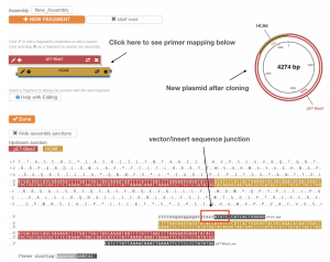
Fig. 2.6. NEBuider displays a predicted plasmid based on input parameters