
39 Orbitals and the 4th Quantum Number, (M7Q6)
Introduction
Learning Objectives for 4th Quantum Number, Orbitals
- Describe orbital shapes and relative energy levels.
| Orbital Shapes | Orbital Energies | - Ascribe and evaluate sets of four quantum numbers.
| Spin Quantum Number | Pauli Exclusion Principle | Summary Table of Quantum Numbers and Significance |
| Key Concepts and Summary | Glossary | End of Section Exercises |
Orbital Shapes
An orbital is the quantum mechanical generalization of Bohr’s orbit. In contrast to his concept of a simple circular orbit with a fixed radius, orbitals are mathematically derived regions of space with different probabilities of having an electron in them.
s-Orbitals
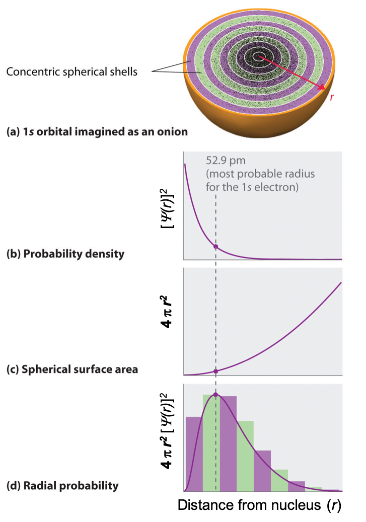
One way of representing electron probability distributions is illustrated in Figure 1 for the 1s orbital of hydrogen. Recall that orbitals are described by wavefunctions, which are represented with ψ. Recall from the M7Q6, that Max Born proposed an interpretation of the wavefunction, ψ, that is still accepted today: the probability density of finding an electron at a given point in space is [ψ(r)]2. In Figure 1a, a dot density diagram is represented. This dot density diagram displays black dots where there is a probability of finding an electron—the higher density of dots, the higher the probability of finding the electron in that region. Taking the information from the dot density diagram, a plot of [ψ(r)]2 versus distance from the nucleus (r) can be constructed. This type of plot (shown in Figure 1b) is a plot of the probability density. This plot shows the probability of finding the electron near a particular point in space that lies a distance r from the nucleus. The 1s orbital is spherically symmetrical, so the probability of finding a 1s electron at any given point depends only on its distance from the nucleus. The probability density is greatest at r = 0 (at the nucleus) and decreases steadily with increasing distance. At very large values of r, the electron probability density is tiny but not exactly zero.
In contrast to the probability density, we can calculate the radial probability (the probability of finding a 1s electron at a distance r from the nucleus) by adding together the probabilities of an electron being at all points on a series of x spherical shells of radius r1, r2, r3,…, rx − 1, rx. In effect, we are dividing the atom into very thin concentric shells, much like the layers of an onion (Figure 1a), and calculating the probability of finding an electron on each spherical shell. Recall that the electron probability density is greatest at r = 0 (Figure 1b), so the density of dots is greatest for the smallest spherical shells in Figure 1a.
The surface area of each spherical shell is equal to 4πr2, which increases rapidly with increasing r (Figure 1c). Because the surface area of the spherical shells increases at first more rapidly with increasing r than the electron probability density decreases, the plot of radial probability has a maximum at a particular distance (Figure 1d). Importantly, when r is very small, the surface area of a spherical shell is so small that the total probability of finding an electron close to the nucleus is very low; at the nucleus, the electron probability vanishes because the surface area of the shell is zero (Figure 1d).
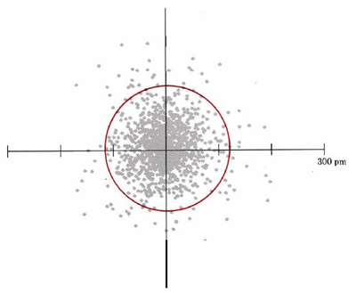
Another representation of the 1s orbital is given in Figure 2. Again, this dot density diagram illustrates the regions where an electron is likely to be found in the “electron cloud”.
Not all s orbitals are the same, however. While the 1s orbital looks like that shown in Figure 2, recall that there are also s orbitals in n = 2, 3, etc. (called 2s, 3s, and ns orbitals). Figure 4 compares the electron probability densities for the hydrogen 1s, 2s, and 3s orbitals. Note that all three are spherically symmetrical. For the 2s and 3s orbitals, however (and for all other s orbitals as well), the electron probability density does not fall off smoothly with increasing r. Instead, a series of minima and maxima are observed in the radial probability plots (Figure 4c). The minima correspond to radial nodes (regions of zero electron probability), which alternate with spherical regions of nonzero electron probability. The orbitals depicted in Figure 4 are of the s type, thus l = 0 for all of them.
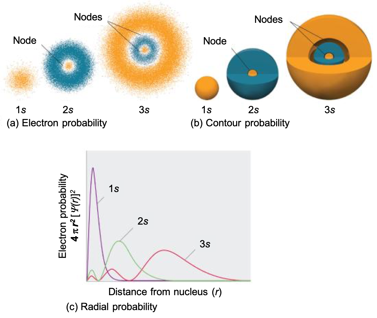
Three things happen to s orbitals as n increases (Figure 4):
- They become larger, extending farther from the nucleus.
- They contain more nodes. This is similar to a standing wave that has regions of significant amplitude separated by nodes (points with zero amplitude). The number of radial nodes in an orbital is n – l – 1.
- For a given atom, the s orbitals also become higher in energy as n increases because of the increased distance from the nucleus.
Orbitals are generally drawn as three-dimensional surfaces that enclose 90% of the electron density. Although such drawings show the relative sizes of the orbitals, they do not normally show the spherical nodes in the 2s and 3s orbitals because the spherical nodes lie inside the 90% surface. Fortunately, the positions of the spherical nodes are not important for chemical bonding. This makes sense because bonding is an interaction of electrons from two atoms which will be most sensitive to forces at the edges of the orbitals.
p-Orbitals
Only s orbitals are spherically symmetrical. As the value of l increases, the number of orbitals in a given subshell increases, and the shapes of the orbitals become more complex. Because the 2p subshell has l = 1, with three values of ml (−1, 0, and +1), there are three 2p orbitals.
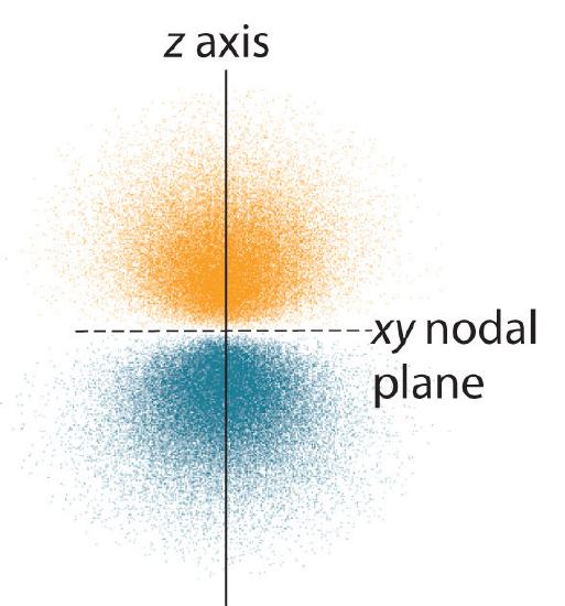
The dot density diagram for one of the hydrogen 2p orbitals is shown in Figure 5. This orbital has two lobes of electron density arranged along the z axis with an electron density of zero in the xy plane. This type of node is called a nodal plane (instead of a radial node which was seen in the s orbitals). Since the xy plane is the nodal plane in Figure 5, it is a 2pz orbital (the orbital is oriented along the z axis).
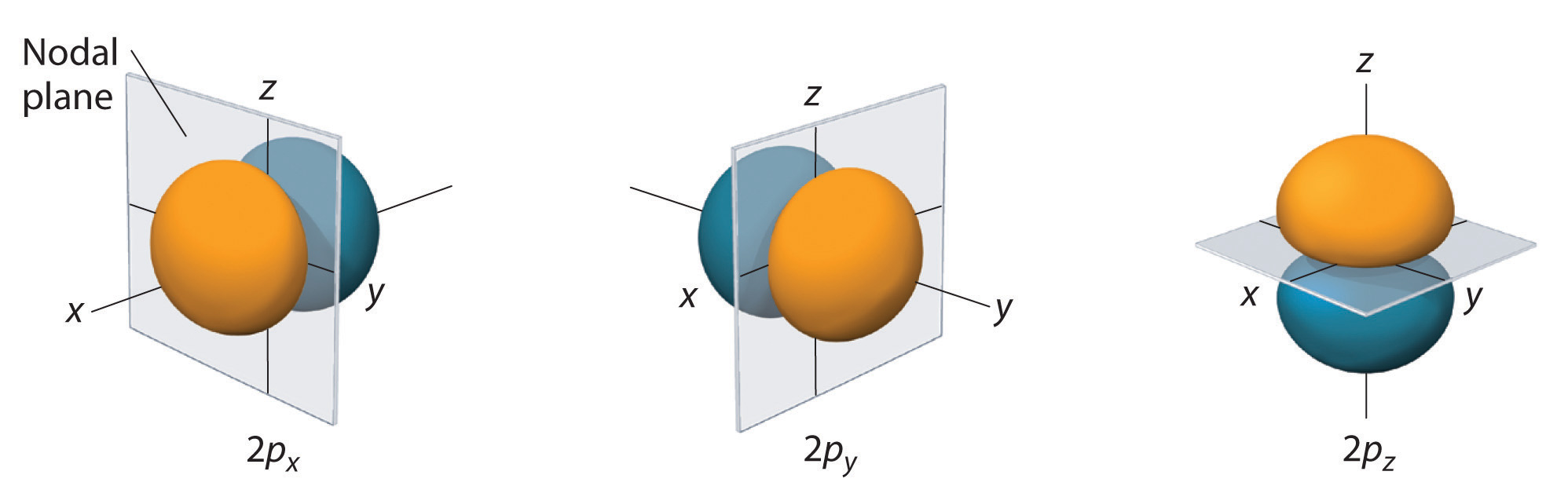
As shown in Figure 6, the other two 2p orbitals have identical shapes, but they lie along the x axis (2px) and y axis (2py), respectively. Note that each 2p orbital has just one nodal plane.
Just as with the s orbitals, the size and complexity of the p orbitals for any atom increase as the principal quantum number n increases. The shapes of the 90% probability surfaces of the 3p, 4p, and higher-energy p orbitals are, however, essentially the same as those shown in Figure 6. The shapes of p orbitals for n > 2 look like strings of beads oriented along the x, y, and z axis with two additional nodes per unit increases in n.
d-Orbitals
Subshells with l = 2 have five d orbitals; the first shell to have a d subshell corresponds to n = 3. The five d orbitals have ml values of −2, −1, 0, +1, and +2.
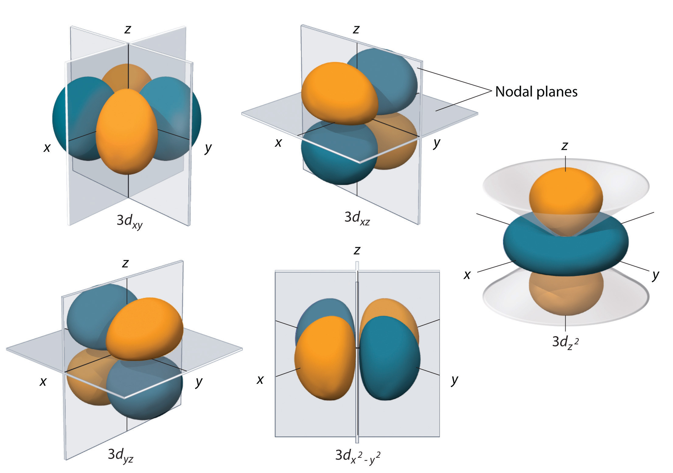
The hydrogen 3d orbitals, shown in Figure 7, have more complex shapes than the 2p orbitals. All five 3d orbitals contain two nodal planes, as compared to one for each p orbital and zero for each s orbital. In three of the d orbitals, the lobes of electron density are oriented between the x and y, x and z, and y and z planes; these orbitals are referred to as the 3dxy, 3dxz, and 3dyz orbitals, respectively. A fourth d orbital has lobes lying along the x and y axes; this is the 3dx2-y2 orbital. The fifth 3d orbital, called the 3dz2 orbital, has a unique shape: it looks like a 2pz orbital combined with an additional doughnut of electron probability lying in the xy plane. Despite its peculiar shape, the 3dz2 orbital is mathematically equivalent to the other four and has the same energy. Like the s and p orbitals, as n increases, the size of the d orbitals increases, but the overall shapes remain similar to those depicted in Figure 7.
f-Orbitals
Principal shells with n = 4 can have subshells with l = 3 and ml values of −3, −2, −1, 0, +1, +2, and +3. These subshells consist of seven f orbitals. Although these orbitals play an important role in the heavier elements, their shapes are complicated and we will not consider these shapes in this course
Orbital Energies
Although we have discussed the shapes of orbitals, we have said little about their comparative energies. We begin our discussion of orbital energies by considering atoms or ions with only a single electron (such as H or He+). This is the simplest case.
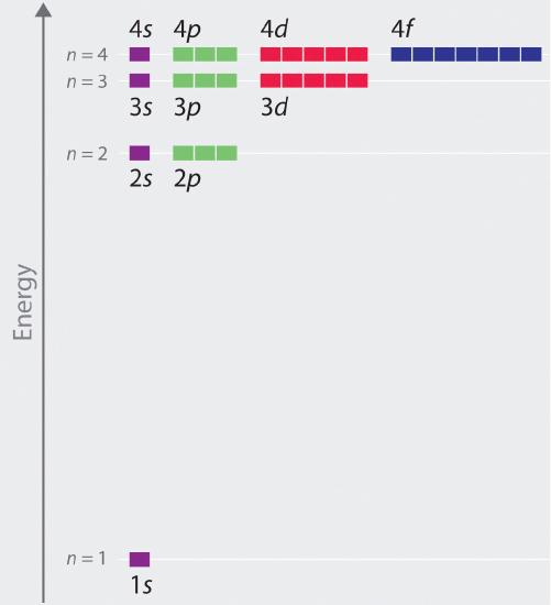
The relative energies of the atomic orbitals with n ≤ 4 for a hydrogen atom are plotted in Figure 8. Note that the orbital energies depend on only the principal quantum number n, not on l. Consequently, the energies of the 2s and 2p orbitals of hydrogen are the same; the energies of the 3s, 3p, and 3d orbitals are the same; and so forth. The orbital energies obtained for hydrogen using quantum mechanics are exactly the same as the allowed energies calculated by Bohr. In contrast to Bohr’s model, however, which allowed only one orbit for each energy level, quantum mechanics predicts that there are 4 orbitals with different electron density distributions in the n = 2 principal shell (one 2s and three 2p orbitals), 9 in the n = 3 principal shell, and 16 in the n = 4 principal shell. As we have just seen, quantum mechanics predicts that in the hydrogen atom, all orbitals with the same value of n (e.g., the three 2p orbitals) are degenerate, meaning that they have the same energy. Figure 8 shows that the energy levels become closer and closer together as the value of n increases, as expected because of the 1/n2 dependence of orbital energies.
Spin Quantum Number
It was demonstrated in the 1920s that when hydrogen line spectra (which we saw previously) are examined at extremely high resolution, some lines are actually not single peaks but rather pairs of closely spaced lines. This is the so-called fine structure of the spectrum, and it implies that there are additional small differences in energies of electrons even when they are located in the same orbital. These observations led Samuel Goudsmit and George Uhlenbeck to propose that electrons have a fourth quantum number. They called this the spin quantum number, or ms.
The other three quantum numbers—n, l, and ml—are properties of specific atomic orbitals that define the most likely location in space of an electron. These orbitals are a result of solving the Schrödinger equation for electrons in atoms. The electron spin is a different kind of property. It is a completely quantum phenomenon with no analogues in the classical realm. In addition, it cannot be derived from solving the Schrödinger equation and is not related to the normal spatial coordinates (such as the Cartesian x, y, and z). Electron spin describes an intrinsic electron “rotation” or “spinning.” Each electron acts as a tiny magnet, just as if it were a tiny rotating object charged with an angular momentum, even though this rotation cannot be observed in terms of the spatial coordinates.
The magnitude of the overall electron spin can only have one value, and an electron can only “spin” in one of two quantized states. One is termed the α state, with the z component of the spin being in the positive direction of the z axis. This corresponds to the spin quantum number ms = +½. The other is called the β state, with the z component of the spin being negative and ms = -½. Any electron, regardless of the atomic orbital it is located in, can only have one of those two values of the spin quantum number. The energies of electrons having ms = -½ and ms = ½ are different if an external magnetic field is applied.
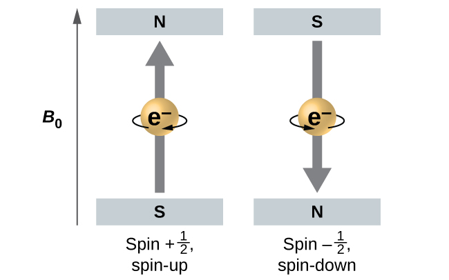
Figure 9 illustrates this phenomenon. An electron acts like a tiny magnet. Its moment is directed up (in the positive direction of the z axis) for the +½ spin quantum number and down (in the negative z direction) for the -½ spin quantum number. A magnet has a lower energy if its magnetic moment is aligned with the external magnetic field (the left electron in Figure 19) and a higher energy for the magnetic moment being opposite to the applied field. This is why an electron with ms = +½ has a slightly lower energy in an external field in the positive z direction, and an electron with ms = -½ has a slightly higher energy in the same field. This is true even for an electron occupying the same orbital in an atom. A spectral line corresponding to a transition for electrons between the same orbitals but with different spin quantum numbers has two possible values of energy; thus, the line in the spectrum will show a fine structure splitting.
The Pauli Exclusion Principle
An electron in an atom is completely described by four quantum numbers: n, l, ml, and ms. The first three quantum numbers define the orbital and the fourth quantum number describes the intrinsic electron property called spin. An Austrian physicist Wolfgang Pauli formulated a general principle that gives the last piece of information that we need to understand the general behavior of electrons in atoms. The Pauli exclusion principle can be formulated as follows: No two electrons in the same atom can have exactly the same set of all four quantum numbers. What this means is that electrons can share the same orbital (the same set of the quantum numbers n, l, and ml), but only if their spin quantum numbers, ms, have different values. Since the spin quantum number can only have two values (± ½), no more than two electrons can occupy the same orbital (and if two electrons are located in the same orbital, they must have opposite spins). Therefore, any atomic orbital can be populated by only zero, one, or two electrons.
The properties and meaning of the quantum numbers of electrons in atoms are briefly summarized in Table 1.
| Name | Symbol | Allowed values | Physical meaning |
|---|---|---|---|
| principal quantum number | n | 1, 2, 3, 4, …. | shell, the general region of an electron in the orbital (distance away from the nucleus) |
| azimuthal (or angular momentum) quantum number | l | 0 ≤ l ≤ n – 1 | subshell, the shape of the orbital |
| magnetic quantum number | ml | – l ≤ ml ≤ l | orientation of the orbital |
| spin quantum number | ms | +½, −½ | direction of the intrinsic quantum “spinning” of the electron |
| Table 1. Quantum numbers, their properties, and significance | |||
Example 1
Maximum Number of Electrons
Calculate the maximum number of electrons that can occupy a shell with (a) n = 2, (b) n = 5, and (c) n as a variable. Note you are only looking at the orbitals with the specified n value, not those at lower energies.
Solution
(a) When n = 2, there are four orbitals (a single orbital with l = 0, and three orbitals labeled l = 1). These four orbitals can contain eight electrons.
(b) When n = 5, there are five subshells of orbitals that we need to sum:
Again, each orbital holds two electrons, so 50 electrons can fit in this shell.
(c) The number of orbitals in any shell n will equal n2. There can be up to two electrons in each orbital, so the maximum number of electrons will be 2 × n2
Check Your Learning
If a shell contains a maximum of 32 electrons, what is the principal quantum number, n?
Answer:
n = 4
Key Concepts and Summary
The azimuthal quantum number determines the general shape of the orbital. For l = 0 (an s orbital), the orbital is spherical. For l = 1 (p orbitals), there are three different p orbitals, but they all have a dumbbell shape. Different ml values are used to differentiate between the three orbitals. The d orbitals, with l = 2, generally have a four-lobed shape. As the n value increases, so does the complexity of the orbitals in each subshell. The first three quantum numbers describe these orbitals. The fourth quantum number is the spin quantum number. Each electron has a spin quantum number, ms, that can be equal to ±½. No two electrons in the same atom can have the same set of values for all the four quantum numbers, known as the Pauli exclusion principle. A consequence of the Pauli exclusion principle is that each orbital can hold at most two electrons.
Glossary
- degenerate orbitals
- orbitals with the same energy level
d orbital
region of space with high electron density that is either four lobed or contains a dumbbell and torus shape; describes orbitals with l = 2. An electron in this orbital is called a d electron
-
- f orbital
- multilobed region of space with high electron density, describes orbitals with l = 3. An electron in this orbital is called an f electron
-
- p orbital
- dumbbell-shaped region of space with high electron density, describes orbitals with l = 1. An electron in this orbital is called a p electron
-
- Pauli exclusion principle
- specifies that no two electrons in an atom can have the same value for all four quantum numbers
- s orbital
- spherical region of space with high electron density, describes orbitals with l = 0. An electron in this orbital is called an s electron
spin quantum number (ms)
number specifying the electron spin direction, either +½ or -½
Chemistry End of Section Exercises
- Consider the orbitals shown here in outline.
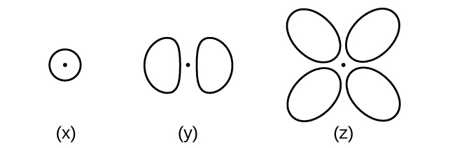
- What is the maximum number of electrons contained in an orbital of type (x)? Of type (y)? Of type (z)?
- How many orbitals of type (x) are found in a shell with n = 2? How many of type (y)? How many of type (z)?
- Write a set of quantum numbers for an electron in an orbital of type (x) in a shell with n = 4. Of an orbital of type (y) in a shell with n = 2. Of an orbital of type (z) in a shell with n = 3.
- What is the smallest possible n value for an orbital of type (x)? Of type (y)? Of type (z)?
- What are the possible l and ml values for an orbital of type (x)? Of type (y)? Of type (z)?
- What are the allowed values for each of the four quantum numbers: n, l, ml, and ms?
- How many electrons could be held in the second shell of an atom if the spin quantum number ms could have three values instead of just two? (Hint: Consider the Pauli exclusion principle.)
- Write a set of quantum numbers for each of the electrons with an n of 4 in a Se atom.
- Identify the subshell in which electrons with the following quantum numbers are found:
- n = 2, l = 1
- n = 4, l = 2
- n = 6, l = 0
- Identify the subshell in which electrons with the following quantum numbers are found:
- n = 3, l = 2
- n = 1, l = 0
- n = 4, l = 3
Answers to Chemistry End of Section Exercises
- (a) x. 2, y. 2, z. 2; (b) x. 1, y. 3, z. 0; (c) x. 4 0 0, y. 2 1 0, z. 3 2 0; (d) x. 1, y. 2, z. 3; (e) x. l = 0, ml = 0, y. l = 1, ml = –1, 0, or +1, z. l = 2, ml = –2, –1, 0, +1, +2
- n = 1, 2, 3…, l = 0, … n-1, ml = –l, … l, ms = -½, +½
- 12
-
n l ml ms 4 0 0 +½ 4 0 0 -½ 4 1 −1 +½ 4 1 0 +½ 4 1 +1 +½ 4 1 −1 -½ Table 4. - (a) 2p; (b) 4d; (c) 6s
- (a) 3d; (b) 1s; (c) 4f
