
Unit Three
Day 20: Rate of Radioactive Decay
D20.1 Radioactive Decay
Determining the rate law and rate constant of a reaction has numerous real world applications, one of which involves the rate of radioactive decay, the spontaneous change of an unstable nuclide into a different nuclide. (A nuclide is an atomic species of a specific isotope; all examples of a given nuclide have the same number of protons and the same number of neutrons.) The rate of radioactive decay allows scientists to learn about the histories of our world in geological and archaeological studies. Before we get to the kinetics of radioactive decay, let’s first consider what reactions are involved in radioactive decay.
During a radioactive decay process, the unstable nuclide is called the parent nuclide; the nuclide that results from the decay is called the daughter nuclide (Figure 1). The daughter nuclide may be stable, or it may decay itself.
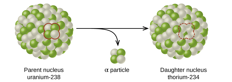
The atomic representations used when discussing radioactive decay reactions have two numbers written to the left of the atomic symbol, for example, [latex]^{238}_{\;92}\text{U}[/latex] and its isotope [latex]^{235}_{\;92}\text{U}[/latex]. The subscript denotes the atomic number, Z, of the element (number of protons), and the superscript denotes the mass number, A, of the isotope (number of protons + number of neutrons). Both subscript and superscript are necessary for balancing nuclear equations.
Exercise 1: Atoms and Isotopes
D20.2 Types of Radioactive Decay
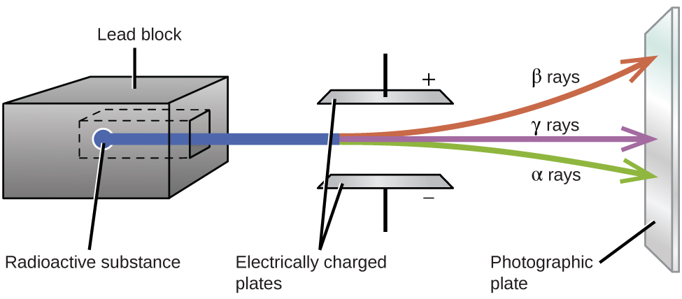
Experiments involving the interaction of radiation with a magnetic or electric field (Figure 2) indicated that one type of radioactive decay particle consists of positively charged and relatively massive α particles, which are high-energy helium nuclei ([latex]_2^4\text{He}[/latex], or [latex]_2^4{\alpha}[/latex]); a second type consists of negatively charged and much lighter β particles, which are high-energy electrons ([latex]_{-1}^{\;\;0}{\beta}[/latex], or [latex]_{-1}^{\;\;0}\text{e}[/latex]); and a third consists of uncharged electromagnetic waves, γ rays, which are very high energy photons. (Note that for β particles, which do not contain any protons, the subscript denotes the charge of the particle.) These three types of radioactive decays are the most commonly observed ones.
α decay is the emission of an α particle from the nucleus. For example:
α decay occurs primarily in heavy nuclei (A > 200, Z > 83). The loss of an α particle gives a daughter nuclide with a mass number four units smaller and an atomic number two units smaller than those of the parent nuclide. Note that the sum of protons (subscripts) on the product side is equal to that on the reactant side. The same is true for the mass number (superscripts). This nuclear reaction is balanced.
β decay is the emission of an electron from a nucleus. For example:
Beta decay involves the conversion of a neutron into a proton and a β particle. The β particle emitted is from the atomic nucleus and is not one of the electrons surrounding the nucleus. Emission of a β particle does not change the mass number of the nuclide but does increase its number of protons and decrease its number of neutrons.
γ decay is the emission of a γ-ray photon from a nucleus. The energies of γ rays are quite high, in the range of 105-107 kJ/mol, so γ rays can easily break chemical bonds if they are absorbed by matter. (In comparison, x-rays have energies roughly 10 times smaller than γ rays.) Cobalt-60 is a nuclide that decays via β emission as well as γ emission:
The asterisk (*) denotes that the nickel-60 produced in the above radioactive decay is in an excited state. It decays to its ground state with the emission of another γ photon:
There is no change in mass number or atomic number during γ emission unless it is accompanied by one of the other modes of decay.
Positron (β+) decay is the emission of a positron, or antielectron, from a nucleus. In the process, a proton is converted into a neutron. For example:
Electron capture occurs when one of the inner electrons in an atom is captured by the atom’s nucleus and transforms a proton into a neutron. For example:
Electron capture has the same effect on the nucleus as does β+ decay, and both are sometimes considered as a type of β decay.
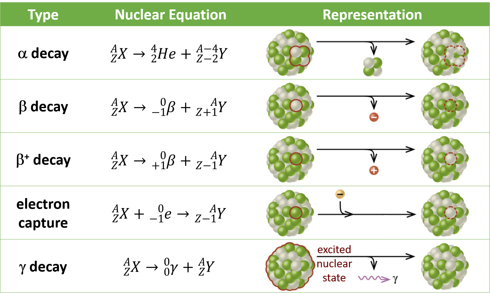
The table below summarizes the various types of radioactive decay.
Exercise 2: Radioactive Decay
Exercise 3: Radioactive Decay and Transmutation of Elements
D20.3 Half-Life of a Reaction
An important aspect of the kinetics of radioactive decay is the half-life (t½) of the reaction, which is the time required for the concentration of a reactant (e.g. the parent nuclide) to be reduced to half of its initial value. In each succeeding half-life, the remaining concentration of the reactant is again halved.
The half-life of a reaction can be derived from the integrated rate law. Hence, there is a general equation for half-life for zeroth-order, first-order, and second-order reaction.
First-Order Reaction
The integrated rate law gives:
When t = t½:
Therefore:
The half-life of a first-order reaction is inversely proportional to the rate constant k: A fast reaction (larger k) has a shorter half-life; a slow reaction (smaller k) has a longer half-life. Moreover, the half-life is, conveniently, independent of the concentration of the reactant. Therefore, you do not need to know the initial concentration to calculate the rate constant from the half-life, or vice versa.
Exercise 4: Half-Life, Rate, and Concentration
Second-Order Reactions
The integrated rate law is:
When t = t½, [latex][\text{A}]_{t_{\frac{1}{2}}} = \frac{1}{2}[\text{A}]_0[/latex], so
Therefore:
For a second-order reaction, t½ is inversely proportional to the rate constant and the concentration of the reactant, and hence is not constant throughout the reaction. The half-life increases as the reaction proceeds due to decreasing concentration of reactant. Consequently, unlike the situation with first-order reactions, the rate constant of a second-order reaction cannot be calculated directly from the half-life unless the initial concentration is known.
Zeroth-Order Reactions
For a zeroth-order reaction:
When t = t½, [latex][\text{A}]_{t_{\frac{1}{2}}} = \frac{1}{2}[\text{A}]_0[/latex], so
The half-life of a zeroth-order reaction is inversely proportional to the rate constant and directly proportional to the concentration of the reactant. Therefore, t½ decreases as the reaction progresses and the reactant concentration decreases.
Activity 1: Half-life and Order from Concentration-Time Data
Exercise 5: Half-life from Rate Constant
D20.4 Radioactive Half-Lives
Radioactive decay occurs in atomic nuclei and therefore does not depend on chemical bonding or collisions of molecules. Therefore, most radioactive decay processes follow first-order kinetics, and have a characteristic, constant half-life. A radioactive isotope’s half-life allows us to determine how long a sample of a useful isotope will be available, or how long a sample of an undesirable or dangerous isotope must be stored before it decays to a sufficiently low radiation level.
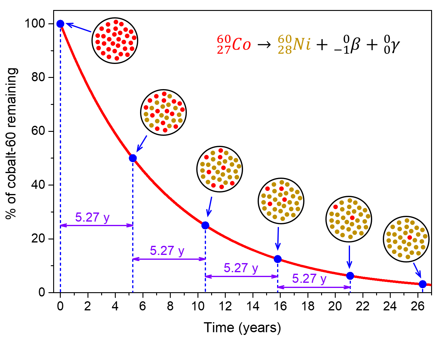
For example, cobalt-60, an isotope that emits gamma rays used to treat cancer, has t½ = 5.27 years (Figure 3). Therefore, in a given cobalt-60 source, both the amount of [latex]_{27}^{60}\text{Co}[/latex] and the intensity of the radiation emitted is cut in half every 5.27 years.
The number of nuclear transformations per unit time is called the activity, symbol A, of the radioactive sample. The activity of a sample can be measured with an instrument, such as a Geiger counter. The activity is directly proportional to the number of radioactive nuclei present, which is symbolized by N. The rate constant for nuclear decay is called the decay constant, symbol λ. Hence, the rate expression for radioactive decay becomes:
This is analogous to the first-order rate law for a chemical reaction, X → products,
Rate = [latex]-\dfrac{\Delta \text{[X]}}{\Delta t} = k[X][/latex]
but the rate is called the activity and the concentration of reactant is replaced by the number of radioactive nuclei. Because the radioactivity is defined in terms of the number of radioactive nuclei, the activity increases as the mass of a sample of radioactive material increases.
The other kinetic equations for first-order reactions similarly apply to radioactive decay, but with the radioactive-decay-specific symbols:
Note that rather than concentration units (M or mol/L), N0 and Nt have the units of moles or number of atoms.
Activity 2: Radioactive Decay and Half-life
Exercise 6: Mass of Radioactive Nuclide Remaining
D20.5 Radiometric Dating
Several radioisotopes have half-lives and other properties that make them useful for radiometric dating, the process of determining an object’s date of origin. The objects of interest can be geological formations, archaeological artifacts, or formerly living organisms. Radiometric dating has been responsible for many breakthrough scientific discoveries about the geological history of the earth, the evolution of life, and the history of human civilizations.
Radiometric Dating Using Carbon-14
Radiocarbon dating or carbon-14 dating can provide reasonably accurate dating of carbon-containing substances up to ~50,000 years old.
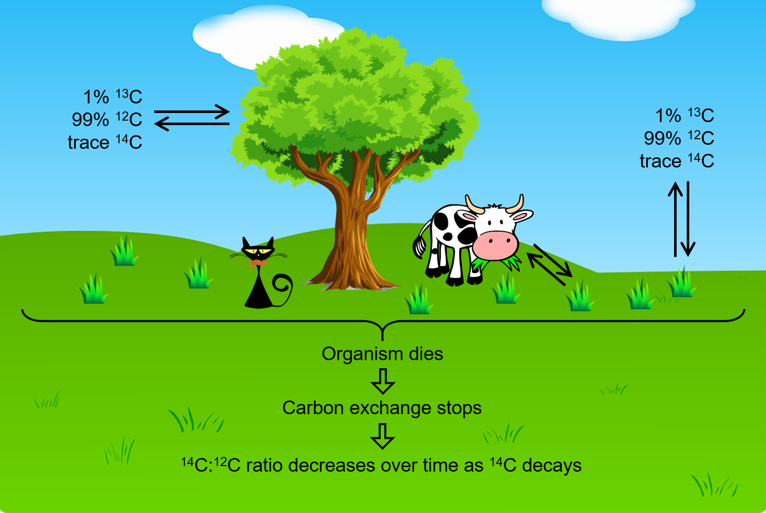
Naturally occurring carbon consists of three isotopes: 12C, which constitutes 99% of the carbon on earth; 13C, about 1% of the total; and 1 part per trillion (0.0000000001%) of 14C. 14C is formed in the upper atmosphere by the reaction of nitrogen atoms with neutrons:
All isotopes of carbon react with oxygen to produce CO2. In the atmosphere, the ratio of 14CO2 to 12CO2 has been nearly constant for a long time, as shown by analysis of carbon-containing gas samples trapped in Greenland ice sheets.
The incorporation of 14CO2 and 12CO2 into plants is a regular part of photosynthesis. Therefore, a living plant is constantly exchanging carbon with its environment, meaning that the [latex]\frac{^{14}\text{C}}{^{12}\text{C}}[/latex] ratio found in a living plant is the same as the [latex]\frac{^{14}\text{C}}{^{12}\text{C}}[/latex] ratio in the atmosphere. But when a plant dies, the carbon exchange with the atomosphere stops. Because 12C is a stable isotope and does not undergo radioactive decay, the amount of 12C in the dead plant does not change. However, 14C undergoes β decays with a half-life of 5730 years:
Thus, the [latex]\frac{^{14}\text{C}}{^{12}\text{C}}[/latex] ratio gradually decreases after the plant dies, and this provides a measure of the time that has elapsed since the death of the plant. For example, if the [latex]\frac{^{14}\text{C}}{^{12}\text{C}}[/latex] ratio in a wooden object found in an archaeological site is half what it is in a living tree, this indicates that 5730 years have elapsed since the death of the tree from which the wooden object was made. Highly accurate determinations of [latex]\frac{^{14}\text{C}}{^{12}\text{C}}[/latex] ratios can be obtained from very small samples (as little as a milligram) by the use of a mass spectrometer.
This process works for other organisms as well, since they also constantly exchange carbon (by eating plants or eating others that eat plants) until they die.
Activity 3: Radiocarbon Dating
The accuracy of radiocarbon dating assumes that the [latex]\frac{^{14}\text{C}}{^{12}\text{C}}[/latex] ratio in a living plant is the same now as it was in an earlier era, but this is not always valid. For example, right now, due to the increasing accumulation of CO2 (largely 12CO2) in the atmosphere, caused by combustion of fossil fuels in which essentially all of the 14C has decayed, the [latex]\frac{^{14}\text{C}}{^{12}\text{C}}[/latex] ratio in our atmosphere is decreasing. This in turn affects the [latex]\frac{^{14}\text{C}}{^{12}\text{C}}[/latex] ratio in currently living organisms on the earth. Fortunately, we can use other data, such as tree dating via examination of annual growth rings, to calculate correction factors. With these correction factors, more accurate dates can be determined. In general, radioactive dating only works for about 10 half-lives; therefore, the limit for carbon-14 dating is about 57,000 years.
Radiometric Dating Using Nuclides Other than Carbon-14
Radiometric dating using radioactive nuclides with half-lives longer than that of carbon-14 can date events older than 57,000 years ago.
For example, uranium-238 can be used to estimate the ages of some of the oldest rocks on earth. Since 238U has a half-life of 4.5 billion years, it takes that amount of time for half of the original 238U to decay by a series of nuclear reactions into 206Pb. In a rock sample that does not contain appreciable qunatities of 208Pb, the most abundant isotope of lead, we can assume that lead was not present when the rock was formed. Therefore, by measuring and analyzing the ratio of [latex]\frac{^{238}\text{U}}{^{206}\text{Pb}}[/latex], we can determine the age of the rock. This assumes that all of the 206Pb present came from the decay of 238U. If there is 206Pb from sources other than 238U, which is often indicated by the co-presence of other lead isotopes in the sample, it is necessary to make adjustments in the calculations.
Potassium-argon dating uses a similar method. 40K decays to form 40Ar with a half-life of 1.25 billion years. If a rock sample is crushed and the amount of 40Ar gas that escapes is measured, determination of the [latex]\frac{^{40}\text{K}}{^{40}\text{Ar}}[/latex] ratio yields the age of the rock. Other methods, such as rubidium-strontium dating (87Rb decays into 87Sr with a half-life of 48.8 billion years), operate on the same principle.
To estimate the lower limit for the earth’s age, scientists determine the age of various rocks and minerals, making the assumption that the earth is older than the oldest rocks and minerals in its crust. As of 2014, the oldest known rocks on earth are the Jack Hills zircons from Australia, found by uranium-lead dating to be almost 4.4 billion years old.
Day 20 Pre-class Podia Problem: Radiocarbon Dating
A sample of an igneous rock contains 9.58 × 10⁻⁵ g of 238U, 2.51 × 10⁻⁵ g of 206Pb, and a negligible quantity of 208Pb. No other lead isotopes are detected. Determine the approximate time at which the rock was formed. (238U decays into 206Pb with a half-life of 4.5 × 10⁹ y.)
Two days before the next whole-class session, this Podia question will become live on Podia, where you can submit your answer.
