
Unit One
Day 4: Periodic Trends; Forces between Atoms
In addition to atomic radius, several other properties vary depending on position in the periodic table. Like atomic radius, these properties depend on effective nuclear charge and size of atomic shell.
D4.1 Periodic Variation in Ionization Energies
The quantum mechanics model for the hydrogen atom (Section D2.4) discussed ionization of the hydrogen atom: excitation of the electron from the n = 1 level to the limit of n → ∞:
Ionization energy (IE), the minimum energy required to remove an electron from the atomic orbital it occupies (exciting it to n = ∞), also applies to multi-electron atoms. As shown in this table of ionization energies, there are successive ionization energies, one for each electron.
The first ionization energy (IE1) is the minimum energy required to remove the least tightly bound electron, i.e. the electron in the highest energy orbital. It corresponds to the process:
The second ionization energy (IE2) is the minimum energy required for removing an electron from the 1+ cation, corresponding to:
And so forth.
Electrons in atoms have lower potential energy than when separated from the atom, so energy is always required to remove the electrons from atoms or ions. Ionization is an endothermic process and IE values are always positive.
Ionization energies can be determined experimentally from atomic spectra or by shining light on a gas-phase sample and successively increasing the photon energy until ejection of an electron is observed. Such experiments also give us direct information about the atomic orbital the electron was occupying.
Exercise 1: Periodic Variation of Ionization Energy
In the preceding activity, you developed a general rule that across a period, IE1 increases with increasing atomic number, Z; down a group, IE1 decreases with increasing Z. Look at Figure 1 below and make certain you see how the data in the figure support both trends. There are a few systematic deviations from these trends, which also can be seen in Figure 1.
Examine data presented in Figure 1. Identify all deviations from the trend that ionization energy increases across a period and decreases down a group. Click on each deviation involving an element in Period 1, Period 2, or Period 3.
Another deviation occurs when a subshell becomes more than half filled. For example, oxygen’s IE1 is slightly lower than that for nitrogen. The orbital diagram of oxygen shows that the last electron added (red) is forced to pair with another electron, because the 2p subshell is more than half full.
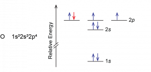
Loss of the electron (colored red in the orbital diagram) yields a greater reduction of electron–electron repulsion because there are no longer two electrons in the same orbital. This makes it easier to lose one electron from O and the ionization energy is smaller than expected. The same explanation applies to the dip for sulfur after phosphorus in Figure 1.
Looking at the successive IEs in the appendix, we see that for any element, IE1 < IE2 < IE3, and so forth, and this is due to the greater Zeff in successively more positive ions. However, sometimes the increase in successive IE is larger than expected. For example, consider the data in Table 1:
| Element | IE1 | IE2 | IE3 | IE4 | IE5 | IE6 | IE7 |
|---|---|---|---|---|---|---|---|
| K | 419 | 3069 | 4438 | 5876 | 7975 | 9620 | 11385 |
| Ca | 590 | 1145 | 4941 | 6465 | 8142 | 10496 | 12350 |
| Sc | 633 | 1244 | 2388 | 7130 | 8877 | 10720 | 13314 |
| Ga | 579 | 1982 | 2962 | 6194 | 8299 | 10874 | 13585 |
| Ge | 760 | 1537 | 3301 | 4409 | 9012 | 11183 | 13981 |
| As | 947 | 1949 | 2731 | 4834 | 6040 | 12302 | 14183 |
| Table 1. Successive Ionization Energies (IEs) for Some Period-4 Elements (kJ/mol) | |||||||
These observed ionization energies are consistent with the idea of valence electrons—electrons in outer shell(s) that are less bound and more energetically accessible, allowing them to participate in chemical transformations.
D4.2 Periodic Variation in Electron Affinities
Electron affinity (EA) is defined as the change in energy when an electron is added to an atom to form an anion. The first EA corresponds to adding one electron to an atom:
Exercise 2: Ionization Energy vs Electron Affinity
Many elements have negative EA1, which means that the energy of the 1− anion is lower than the energy of the atom plus the free electron; that is, the anion is more stable.
For other elements, EA1 is positive, meaning that the anion is less stable compared to the parent atom plus a free electron. For these elements, an input of energy is required to form the anion, and, in the gas phase, the anion dissociates to yield the neutral atom and a free electron because the latter are lower in energy.
D4.3 Electron Configurations of Monoatomic Ions
When atoms lose electrons or gain electrons, Ions form. It is useful to know what kinds of ions form and what their properties are. A monoatomic ion is a single atom that has gained or lost one or more electrons. A positively charged ion, a cation, forms when an atom loses one or more electrons. A negatively charged ion, an anion, forms when an atom gains one or more electrons.
Nonmetallic elements on the far right side of the periodic table (except the noble gases) have higher ionization energies and more negative electron affinities. It is energetically more favorable for them to gain electrons and form anions and less energetically favorable for them to form cations. For example, elements in groups VIIA, VIA, and some in VA can gain 1, 2, or 3 electrons, respectively, to achieve the electron configuration of a noble gas (a full octet, s2p6 in the outermost shell).
Metallic elements on the left side of the periodic table have lower ionization energies and less negative (or positive) electron affinities. It is energetically more favorable for them to form cations. For examples, elements in groups IA, IIA, and IIIA can lose 1, 2, or 3 electrons, respectively, to achieve a full octet (plus additional filled d and f subshells).
To find the ground state electron configuration of a monoatomic ion, start with the electron configuration of the corresponding atom and remove (or add) an appropriate number of electrons from (or to) the valence orbital(s) of the atom. Here are some examples:
When transition elements and inner transition elements form cations, electron(s) in the outermost shell (largest n) are removed before any d or f electrons. For example, when Fe loses two electrons to form Fe2+, the two 4s electrons are lost:
Exercise 3: Electron Configurations for Monoatomic Ions
In your notebook write the correct electron configuration for each ion listed here:
Sr2+ Te2− Al3+ Fe3+ Nd4+
Exercise 4: Identify Element from Ion Electron Configuration
Ions and atoms that have the same electron configuration are isoelectronic. For example, the isoelectronic Na+, Ne, and F− all have ground state electron configuration of 1s22s22p6 (or [Ne]). For main-group elements, the most commonly formed ions are isoelectronic with a noble gas; that is, these ions have complete octets.
Exercise 5: Isoelectronic Species
D4.4 Unpaired Electrons and Magnetism
One way chemists have discovered information about electron configurations of ions involves magnetism. You are probably familiar with refrigerator magnets, iron magnets, or neodymium (rare earth) magnets. These exhibit ferromagnetism, a strong attraction to a magnetic field that is easily observable and sometimes can be made permanent. All substances exhibit diamagnetism, a very weak repulsion from a magnetic field that can only be observed in extremely large magnetic fields. Because diamagnetism is so weak, it is usually too small to notice.
In addition to diamagnetism, some substances also exhibit paramagnetism, an attraction to a magnetic field that is not as strong as ferromagnetism but much stronger than diamagnetic repulsion. Paramagnetism arises due to the presence of unpaired electrons. Each electron has a tiny magnetic field; that is, each electron is a tiny magnet. When a macroscopic magnet comes near a paramagnetic substance, most of the unpaired electron magnets align with the magnetic field, causing the substance to be attracted to the magnet (Figure 2).
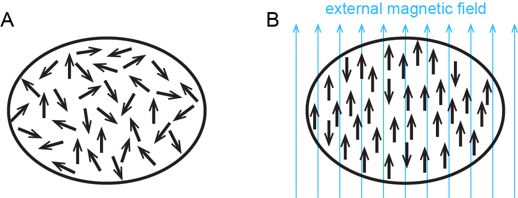
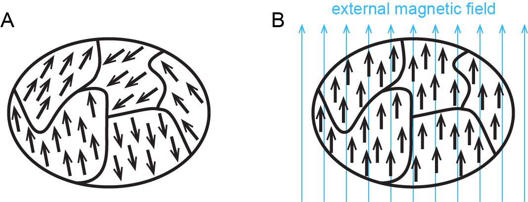
Figure 3 shows how ferromagnetism differs from paramagnetism.
When electrons are paired in an orbital, their opposite magnetic moments create opposite magnetic fields that cancel each other: substances with all electrons paired are neither paramagnetic nor ferromagnetic. They exhibit only diamagnetism and are said to be diamagnetic. For example, argon has a ground state electron configuration of 1s22s22p63s23p6, where each subshell is full and each orbital therein contains a pair of electrons with opposite spins. Hence, a sample of argon is diamagnetic.
Paramagnetic and diamagnetic materials do not act as permanent magnets. A magnetic field is required to align the magnetic moments and make them magnetic. The magnitude of paramagnetism can be measured by weighing a sample with a highly sensitive balance and then weighing it again with a strong magnet just below the sample. A sample that is attracted to the magnet appears heavier because the magnet attracts it downward. The increase in apparent weight is proportional to the number of unpaired electrons.
Exercise 6: Diamagnetic and Paramagnetic Ions
D4.5 Ionic Radii
Ionic radius is the radius of a sphere representing a cation or an anion; it can be determined from structures of ionic crystals.
Cations have fewer electrons than the uncharged atoms from which they are derived. Hence, there is less electron-electron repulsion (that is, larger Zeff), which makes a cation’s radius smaller than the corresponding uncharged atom’s radius. For example, the atomic radius of Al ([Ne]3s23p1) is 143 pm, which is more than twice as large as the 68 pm ionic radius of Al3+ ([Ne]). Often, as in the case of Al, formation of a cation involves removal of all electrons from the outermost shell of an atom, which means the remaining electrons are in a smaller shell—another reason why cations are smaller than the atoms from which they form.
For the same element, cations with larger positive charges are smaller than cations with smaller charges. For example, V2+ has an ionic radius of 93 pm, while that of V3+ is 78 pm. (An uncharged V atom has an atomic radius of 135 pm.)
Anions have more electrons and therefore greater electron-electron repulsion (that is, smaller Zeff) than the neutral atoms from which they are derived. Thus, an anion’s radius is larger than the parent atom’s radius. For example, the ionic radius of S2- ([Ne]3s23p6) is 170 pm, larger than the 104 pm atomic radius of S ([Ne]3s23p4).
Periodic trends in radii of a set of anions (or cations) with the same charge are similar to the atomic-radius trends. For instance, proceeding down a group, radii of 1+ cations generally increase as atomic number increases, corresponding to the increase in the principal quantum number, n.
For isoelectronic species (ions or atoms with the same electron configuration, Section D4.3), the greater the nuclear charge (number of protons), the smaller the atomic/ionic radius. This implies that isoelectronic anions are larger than the neutral atom which is larger than the cations.
Exercise 7: Atomic and Ionic Radii
In Days 2 and 3 and above, we have discussed atomic structure and electron density as well as periodic trends in effective nuclear charge, size of atoms, ionization energies, and electron affinities. All of these are central to understanding properties and chemical reactivity of the elements. Next, we apply those ideas to the noble gases and to metals.
Applying Core Ideas: Two Similar Atoms, Two Very Different Substances
Section D1.5 introduced the idea that atoms, molecules, and oppositely charged ions attract and that their potential energy can be described by a curve that starts at zero when the particles are far apart, falls to a minimum, and increases when the particles are very close together. The depth of the minimum in such a curve can be related to physical properties such as boiling points, because atomic-level particles gain energy as temperature increases.
Consider the boiling points of the first five noble gases in the table below.
| Noble Gas | Atomic Number | Atomic Radius (pm) | Boiling Point (K) |
| He | 2 | 31 | 4.22 |
| Ne | 10 | 68 | 27.1 |
| Ar | 18 | 91 | 87.4 |
| Kr | 36 | 108 | 119.9 |
| Xe | 54 | 126 | 165 |
Based on the boiling point data, for which noble gas is the attraction between particles greatest? Which noble gas has the deepest minimum in its curve of potential energy vs distance between atoms? In your notebook, answer these questions. Then use one set of axes and sketch the potential-energy curve for each of the five noble gases in the table, describe the curves in words and explain why you drew the curves as you did.
Based on the experimental data and the curves you drew, correlate the size of the attraction between atoms with the number of electrons and the size of each atom. Write several sentences in your notebook describing the correlation.
Now consider iron, which has atomic number 26 and atomic radius 126 pm (the same radius as Xe, but fewer electrons). Based on this information, sketch the potential energy curve for iron atoms on the graph you made for the noble gases. Describe the curve in words and explain why you drew the curve as you did.
Does what you predicted for iron make sense?
D4.6 Forces Between Atoms
Based only on experimental data for noble gases, one might predict that iron would be a gas at room temperature, but iron is a solid. Attractive forces between iron atoms must be a lot stronger than attractive forces between noble-gas atoms. To make sense of the difference between xenon and iron, we need a better model for forces between atoms.
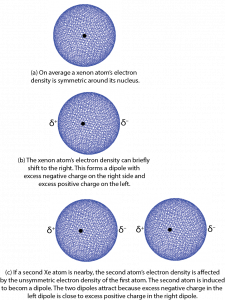
Let’s begin by thinking about attractions between xenon atoms. On average the electron density distribution of the 54 electrons surrounding a xenon nucleus is spherically symmetric. That is, no matter which direction you go from the nucleus, the electron density is the same at the same distance from the nucleus. However, there can be very brief deviations or fluctuations from this average. In 1928 German-American physicist Fritz London used quantum mechanics to show how such fluctuations could lead to attractive forces between atoms and other atomic-scale particles.
Here is a simplified explanation using a Xe atom as an example. Consider a fluctuation in which there is slightly more electron density on one side of the nucleus than on the other. Such a brief deviation creates a dipole, a distribution of electric charge where one side is more positive and the other side is more negative. The dipole only occurs for an instant and is therefore called an instantaneous dipole. This is shown in Figure 4, parts a and b, where δ+ and δ− indicate tiny fractions of the charge of an electron.
If a second Xe atom is close to the first one when the instantaneous dipole forms, for example, on the right of the first one as in Figure 4, part c, the excess negative charge on the right of the first Xe atom repels the electrons on the second Xe atom. This forms a second dipole, again for only an instant. The second dipole is said to be induced by the first one. The positively charged end of the second dipole is attracted to the negatively charged end of the first dipole. For the instant that the dipoles exist, there is a weak attraction between the two atoms.
These weak attractive forces due to instantaneous fluctuations in electron density are called London dispersion forces; we will often refer to them as LDFs. LDFs are present between all atomic-scale particles: atoms, molecules, and ions. The size of the attractive force depends on the number of electrons in a particle and how easily the electron density distribution can be distorted from its average shape.
D4.7 Metals
Based on iron’s boiling point of 3135 K (2862 °C), the forces between iron atoms must be much greater than just LDFs. What you have already learned about atomic structure, effective nuclear charge, and valence electrons can be used to make sense of the much larger forces that attract iron atoms, as well as atoms of other metals.
Metals, which include most of the elements in the periodic table (Figure 5), have characteristic macroscopic properties: they conduct heat and electricity well when they are solids or liquids; they have lustrous (metallic-looking) solid surfaces; and they deform, rather than shatter, when hammered (they are malleable). Many metals are hard, quite strong, and useful as construction materials. What gives rise to these characteristics?

Metallic substances are made of atoms whose valence electron(s) can be removed with relatively low quantities of energy; that is, elements with relatively low ionization energies. Valence electrons of metals experience lower effective nuclear charge than valence electrons of nonmetals; hence, metals tend to form positive ions and nonmetals tend to form negative ions.
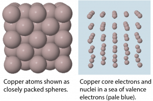
In a metallic solid, atoms are packed closely (Figure 6). One model describes solid metals at the atomic scale as atoms surrounded by mobile valence electrons—a so-called “sea” of electrons. Each “atom” consists of the nucleus and core electrons; that is, a positively charged ion that has lost all its valence electrons. The loosely-bound valence electrons are shared (delocalized) among many different atoms. Electrostatic attractions between the sea of shared valence electrons and the metal ions is known as metallic bonding. The strength of metallic bonding increases as the number of valence electrons shared in the electron sea increases.
Because the valence electrons are delocalized over many metal atoms, if one atom moves relative to others, the attraction between valence electrons and atomic cores remains; that is metallic bonding is not specific to a particular direction. This characteristic accounts for many of the observed physical properties of metals.
Day 4 Pre-Class Podia Problem: Chemical Combinations
This Podia problem is based on today’s pre-class material; working through that material will help you solve the problem.
When nonmetals combine with other nonmetals, compounds form with subscripts that are small whole numbers, such as CO and CO2. When metals combine with nonmetals, formulas of compounds are analogous, such as FeCl2 and FeCl3. When metals combine with other metals, however, they form alloys, substances that have metallic properties but can consist of many different compositions. For example, sodium and potassium can form alloys in which the ratio of sodium atoms to potassium atoms varies from all sodium to all potassium. Thus, if you wrote a formula for sodium-potassium alloy as NaxK, x could have any value from zero to infinity.
Think about why metals should be different in this way. Then write an explanation for the different behavior.
Two days before the next whole-class session, this Podia question will become live on Podia, where you can submit your answer.
