
Unit Four
Day 28: Entropy, Gibbs Free Energy
D28.1 Entropy and Microstates
An important goal of chemical thermodynamics is to predict whether reactants are changed to products or products are changed to reactants. For a given reaction, such a prediction requires knowledge of specific conditions of temperature and of concentrations or partial pressures of reactants and products. When reactants change to products we say that the reaction is spontaneous, or spontaneous in the forward direction. When products change to reactants, we say the reaction is not spontaneous, or that it is spontaneous in the reverse direction. In this context, the word “spontaneous” does not imply that the reaction is fast or slow, just that reactants change to products. Even if it takes millions of years for a process to occur, if there is an overall change of reactants to products we call the process spontaneous.
It is useful to define parallel terms that relate to a convenient reference point—standard-state conditions. If, when all substances are at the standard-state pressure of 1 bar or at the standard-state concentration of 1 M, reactants change to products, we call a reaction product-favored. In contrast, if products change to reactants under standard-state conditions, a process is reactant-favored. That is, a product-favored process is spontaneous under the specific conditions of standard-state pressures or concentrations and a reactant-favored process is not spontaneous under those specific conditions..
Deciding whether a process is spontaneous requires knowledge of the system’s enthalpy change, but that is not sufficient. It also requires knowledge of change in another property: entropy. (Similarly, deciding whether a process is product-favored requires knowledge of the system’s standard enthalpy change and standard entropy change.) The entropy change, ΔS, at constant temperature is defined as:
Here, qrev is the heat transfer of energy for a reversible process, a theoretical process that takes place at such a slow rate that it is always at equilibrium and its direction can be changed (it can be “reversed”) by an infinitesimally small change in some condition. An example of a reversible process is melting water at 0 °C and 1 bar, where liquid water and ice are at equilibrium. Raising the temperature a tiny bit causes the ice to melt; lowering the temperature a tiny bit reverses the process, causing liquid water to freeze.
On a molecular scale, the entropy of a system can be related to the number of possible microstates (W). A microstate is a specific configuration of the locations and energies of the atoms or molecules that comprise a system. The relationship is:
where kB is the Boltzmann constant with a value of 1.38×10⁻²³ J/K.
Similar to enthalpy, the change in entropy for a process is the difference between its final (Sf) and initial (Si) values:
For processes involving an increase in the number of microstates, Wf > Wi, the entropy of the system increases, ΔS > 0. Conversely, processes that reduce the number of microstates, Wf < Wi, yield a decrease in system entropy, ΔS < 0.
Consider the general case of a system comprised of N particles distributed among n boxes. The number of microstates possible for such a system is nN. For example, suppose four atoms, one atom each of He, Ne, Ar, and Kr, are distributed among two boxes as illustrated in Figure 1. There are 24 = 16 different microstates. Microstates with equivalent particle arrangements (not considering individual particle identities) are grouped together and are called distributions. The probability that a system exists as a given distribution is proportional to the number of microstates within the distribution. Because entropy increases logarithmically with the number of microstates, the most probable distribution is the one of greatest entropy.
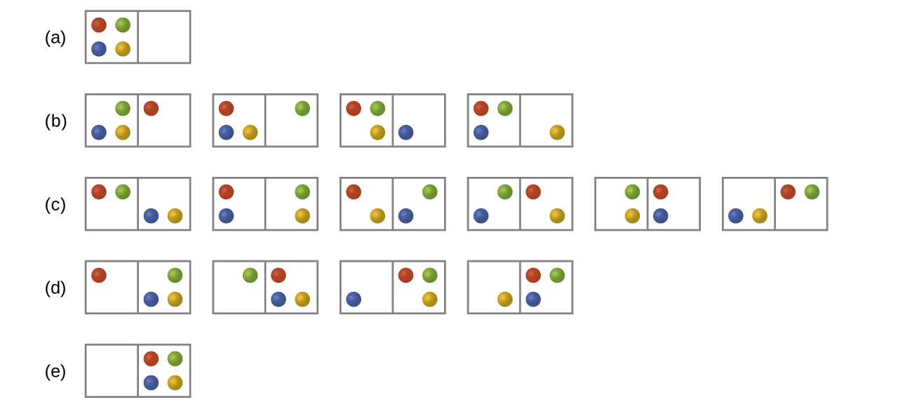
For the system in Figure 1, the most probable distribution is (c), where the particles are evenly distributed between the boxes. The probability of finding the system in this configuration is [latex]\frac{6}{16}[/latex] or 37.5%. The least probable configuration of the system is distributions (a) and (e), where all four particles are in one box, and each distribution has a probability of [latex]\frac{1}{16}[/latex].
As you add more particles to the system, the number of possible microstates increases exponentially (2N). A macroscopic system typically consists of moles of particles (N ≈ 1023), and the corresponding number of microstates is staggeringly huge. Regardless of the number of particles in a system, the distributions with uniform dispersal of particles between the boxes have the greatest number of microstates and are the most probable.
Activity 1: Entropy Change and Microstates
Consider another system as shown in Figure 2. This system consists of two objects, AB and CD, and two units of energy (represented as “*”). Distribution (a) shows the three microstates possible for the initial state of the system, where both units of energy are contained within the hot AB object. If one energy unit is transferred, the result is distribution (b) consisting of four microstates. If both energy units are transferred, the result is distribution (c) consisting of three microstates.
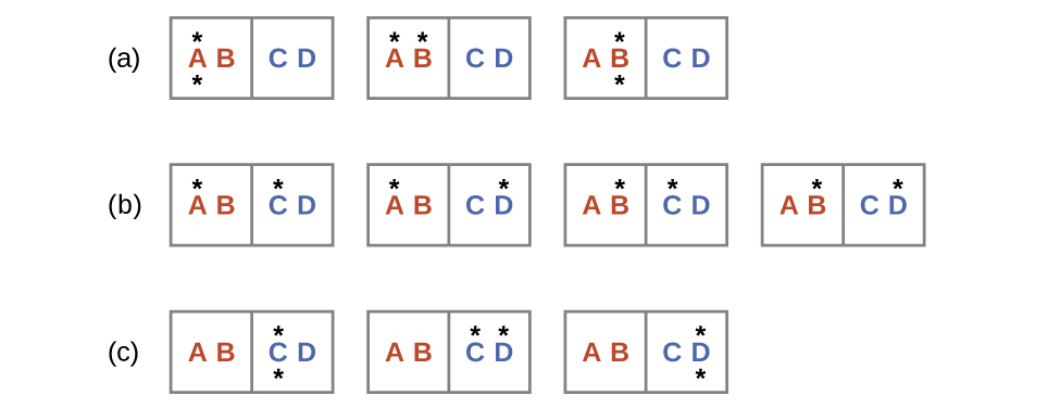
Hence, we may describe this system by a total of ten microstates. The probability that there is no heat transfer of energy when the two objects are brought into contact (the system remains in distribution (a)) is 30%. It is much more likely for heat transfer to occur and yield either distribution (b) or (c), the combined probability being 70%. The most likely result, with 40% probability, is heat transfer to yield the uniform dispersal of energy represented by distribution (b).
This simple example supports the common observation that placing hot and cold objects in contact results in heat transfer that ultimately equalizes the objects’ temperatures. Such a process is characterized by an increase in system entropy.
D28.2 Predicting the Sign of ΔS
The relationships between entropy, microstates, and matter/energy dispersal make it possible for us to assess relative entropies of substances and predict the sign of entropy changes for chemical and physical processes.
Consider the phase changes illustrated in Figure 3. In the solid phase, the molecules are restricted to nearly fixed positions relative to each other and only oscillate a little about these positions; the number of microstates (Wsolid) is relatively small. In the liquid phase, the molecules can move over and around each other, though they remain in relatively close proximity. This increased freedom of motion results in a greater variation in possible particle locations, Wliquid > Wsolid. As a result, Sliquid > Ssolid and the process of melting is characterized by an increase in entropy, ΔS > 0.
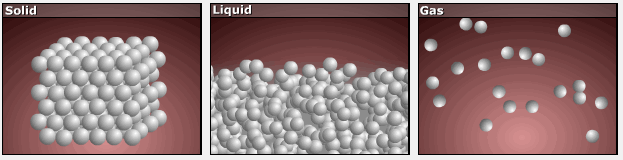
Solids and liquids have surfaces that define their volume, but in the gas phase the molecules occupy the entire container; therefore, for the same sample, each molecule in a gas can be found in many more locations (and there are many more microstates) than in the liquid or solid phase. Consequently, Sgas > Sliquid > Ssolid, and the processes of vaporization and sublimation involve increases in entropy, ΔS > 0.
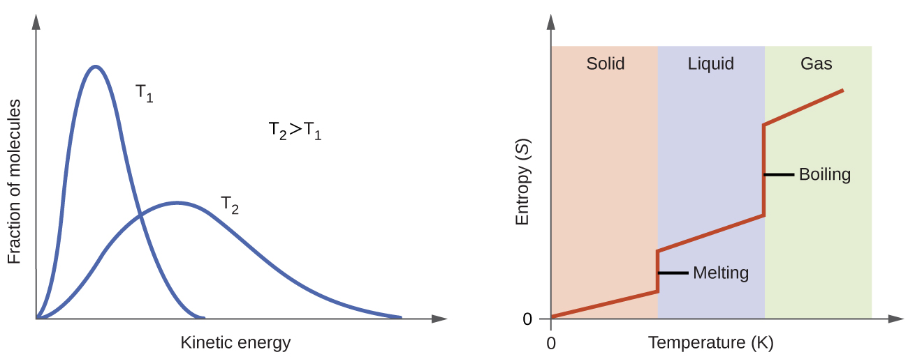
We have already discussed that the temperature of a substance is proportional to the average kinetic energy of its particles. Raising the temperature results in more extensive vibrations of the particles in solids and more rapid movements of the particles in liquids and gases. At higher temperatures, the Maxwell-Boltzmann distribution of molecular kinetic energies is also broader than at lower temperatures; that is, there is a greater range of energies of the particles. Thus, the entropy for any substance increases with temperature (Figure 4).
The entropy of a substance is also influenced by the structure of the particles that comprise the substance. For atomic substances, heavier atoms possess greater entropy at a given temperature than lighter atoms. For heavier atoms the energy levels corresponding to movement from one place to another are closer together, which means that at a given temperature there are more occupied energy levels and more microstates. For molecules, greater number of atoms (regardless of their masses) within a molecule gives rise to more ways in which the molecule can vibrate, which increases the number of possible microstates. Thus, the more atoms there are in a molecule the greater the entropy is.
Finally, variations in the types of particles affects the entropy of a system. Compared to a pure substance, in which all particles are identical, the entropy of a mixture of different particle types is greater due to the additional orientations and interactions that are possible. For example, when a solid dissolves in a liquid, the particles of the solid experience both a greater freedom of motion and additional interactions with the solvent particles. This corresponds to a more uniform dispersal of matter and energy and a greater number of microstates. All other things being equal, the process of dissolution therefore involves an increase in entropy, ΔS > 0.
Exercise 1: Predicting Entropy Changes
D28.3 Second Law of Thermodynamics
The second law of thermodynamics enables predictions of whether a process, such as a chemical reaction, is spontaneous and whether the process is product-favored.
In thermodynamic models, the system and surroundings comprise everything (in other words, the universe), and so
To illustrate this relation, consider the process of heat transfer between two objects, one identified as the system and the other as the surroundings. There are three possibilities for such a process:
- The objects are at different temperatures, and energy transfers from the hotter object to the cooler object. This is always observed to occur. Designating the hotter object as the system and invoking the definition of entropy yields:
[latex]{\Delta}S_{\text{sys}} = \dfrac{-q_{\text{rev}}}{T_{\text{sys}}}\;\;\;\;\;\;\;\text{and}\;\;\;\;\;\;\;{\Delta}S_{\text{surr}} = \dfrac{q_{\text{rev}}}{T_{\text{surr}}}[/latex]
The arithmetic signs of qrev denote the loss of energy by the system and the gain of energy by the surroundings. Since Tsys > Tsurr in this scenario, ΔSsurr is positive and its magnitude is greater than the magnitude of ΔSsys. Thus, ΔSsys and ΔSsurr sum to a positive value for ΔSuniv. This process involves an increase in the entropy of the universe.
- The objects are at different temperatures, and energy transfers from the cooler object to the hotter object. This is never observed to occur. Again designating the hotter object as the system:
[latex]{\Delta}S_{\text{sys}} = \dfrac{q_{\text{rev}}}{T_{\text{sys}}}\;\;\;\;\;\;\;\text{and}\;\;\;\;\;\;\;{\Delta}S_{\text{surr}} = \dfrac{-q_{\text{rev}}}{T_{\text{surr}}}[/latex]
The magnitude of ΔSsurr is again greater than that for ΔSsys, but in this case, the sign of ΔSsurr is negative, yielding a negative value for ΔSuniv. This process involves a decrease in the entropy of the universe. (Note also that possibility 1, which is the reverse of this process, always occurs.)
- The temperature difference between the objects is infinitesimally small, Tsys ≈ Tsurr, and so the heat transfer is thermodynamically reversible. In this case, the system and surroundings experience entropy changes that are equal in magnitude and therefore sum to a value of zero for ΔSuniv. This process involves no change in the entropy of the universe.
These results lead to the second law of thermodynamics: all changes that take place of their own accord (are spontaneous) involve an increase in the entropy of the universe.
| ΔSuniv > 0 | spontaneous (takes place of its own accord) |
| ΔSuniv < 0 | not spontaneous (reverse reaction would occur) |
| ΔSuniv = 0 | system is at equilibrium |
For many realistic applications, the surroundings are vast in comparison to the system. In such cases, the heat transfer of energy to or from the surroundings as a result of some process is a nearly infinitesimal fraction of its total thermal energy. For example, combustion of a hydrocarbon fuel in air involves heat transfer from a system (the fuel and oxygen molecules reacting to form carbon dioxide and water) to surroundings that are significantly more massive (Earth’s atmosphere). As a result, qsurr is a good approximation of qrev, and the second law may be stated as:
We can use this equation to predict whether a process is spontaneous.
Activity 2: Enthalpy, Entropy, and Spontaneous Reactions
D28.4 Third Law of Thermodynamics
Consider the entropy of a pure, perfectly crystalline solid possessing no kinetic energy (that is, at a temperature of absolute zero, 0 K). This system may be described by a single microstate, as its purity, perfect crystallinity and complete lack of motion means there is but one possible location for each identical molecule comprising the crystal (W = 1). According to the Boltzmann equation, the entropy of this system is zero:
This limiting condition for a system’s entropy represents the third law of thermodynamics: the entropy of a pure, perfect crystalline substance at 0 K is zero.
Starting with zero entropy at absolute zero, it is possible to make careful calorimetric measurements (qrev/T) to determine the temperature dependence of a substance’s entropy and to derive absolute entropy values at higher temperatures. (Note that, unlike enthalpy values, the third law of thermodynamics identifies a zero point for entropy; thus, there is no need for formation enthalpies and every substance, including elements in their most stable states, has an absolute entropy.) Standard entropy (S°) values are the absolute entropies per mole of substance at a pressure of 1 bar or a concentration of 1 M. The standard entropy change (ΔrS°) for any chemical process may be computed from the standard entropy of its reactant and product species:
The thermodynamics table in the appendix lists standard entropies of select compounds at 298.15 K.
Exercise 2: Standard Entropy Change
Suppose an exothermic chemical reaction takes place at constant atmospheric pressure. There is a heat transfer of energy from the reaction system to the surroundings, qsurr = –qsys. The heat transfer for the system is the enthalpy change of the reaction because, at constant pressure, ΔrH° = q (Section D27.3). Because the energy transfer to the surroundings is reversible, the entropy change for the surroundings can also be expressed as:
The same reasoning applies to an endothermic reaction: qsys and qsurr are equal but have opposite sign.
Also, for a chemical reaction system, ΔSsys = ΔrS° (the standard entropy change for the reaction). Hence, ΔSuniv can be expressed as:
The convenience of this equation is that, for a given reaction, ΔSuniv can be calculated from thermodynamics data for the system only. That is, from data found in the Appendix.
D28.5 Gibbs Free Energy
A new thermodynamic property was introduced in the late 19th century by American mathematician Josiah Willard Gibbs. The property is called the Gibbs free energy (G) (or simply the free energy), and is defined in terms of a system’s enthalpy, entropy, and temperature:
The change in Gibbs free energy (ΔG) at constant temperature may be expressed as:
ΔG is related to whether a process is spontaneous. This relationship can be seen by comparing to the second law of thermodynamics:
Multiplying both sides of this equation by −T, and rearranging, yields:
Which can be compared to the equation:
Hence:
For a process that is spontaneous, ΔSuniv must be positive. Because thermodynamic temperature is always positive (values are in kelvins), ΔG must be negative for a process that proceeds forward of its own accord.
| ΔSuniv > 0 | ΔGsys < 0 | spontaneous (takes place of its own accord) |
| ΔSuniv < 0 | ΔGsys > 0 | not spontaneous (reverse reaction would occur) |
| ΔSuniv = 0 | ΔGsys = 0 | at equilibrium |
D28.6 Calculating ΔG°
A convenient and common approach to calculate ΔrG° for reactions is by using standard state thermodynamic data. One method involves determining the ΔrH° and ΔrS° first, then using the equation:
Exercise 3: Standard Gibbs Free Energy Change from Enthalpy and Entropy Changes
It is also possible to use the standard Gibbs free energy of formation (ΔfG°) of the reactants and products involved in the reaction to calculate ΔrG°. ΔfG° is the Gibbs free energy change that accompanies the formation of one mole of a substance from its elements in their standard states. It is by definition zero for the most stable form of an elemental substance under standard state conditions.
For a generic reaction:
ΔrG° from ΔfG° would be:
Exercise 4: Calculating Standard Gibbs Free Energy Change
Podia Question
Use data from the Appendix to calculate ΔrS° for this reaction at 298 K:
2 NO(g) + O2(g) → 2 NO2(g)
colorless gas colorless gas → red-brown gas
Predict whether the reaction is product-favored (spontaneous under standard-state conditions) or reactant-favored (not spontaneous under standard-state conditions).
After making your prediction, watch this video where NO(g) is added to O2(g) in a flask:
Does the video validate your prediction? Explain why or why not.
If the video does not validate your prediction, try to figure out why your prediction did not work and re-do it in a different way.
If the video does validate your prediction, explain what thermodynamic aspect of the reaction accounts for the observations in the video.
Two days before the next whole-class session, this Podia question will become live on Podia, where you can submit your answer.
