
Unit One
Day 2: Atomic Spectra and Atomic Orbitals
If you have not yet worked through the Introduction and Day 1, please do so before beginning this section.
D2.1 Electromagnetic Radiation
The periodic table (Section D1.4) summarizes much information about chemical elements. That information can be better understood by assuming that both physical and chemical properties of the different elements depend on differences in the underlying structures of their atoms. An important way to learn about the structures of atoms is to study how energy, in the form of electromagnetic radiation, interacts with matter.
Activity 1: Preparation—Atomic Spectra and Atomic Structure
Electromagnetic radiation consists of oscillating, perpendicular electric and magnetic fields that travel through space and can transfer energy. The oscillating fields (waves) are characterized by wavelength (λ, measured in meters, m) and frequency ([latex]\nu[/latex], measured in hertz, Hz or s−1). In a vacuum, electromagnetic radiation travels at the speed of light (c):
Electromagnetic radiation occurs in small, indivisible quantities of energy called photons. The energy of a photon, Ephoton, can be determined from either its frequency or its wavelength:
[latex]E_{\rm{photon}} = h\nu = \dfrac{{hc}}{\lambda }[/latex]
In this equation h represents Planck’s constant; h = 6.626 × 10⁻³⁴ J s.
Exercise 1: Photon Energy from Wavelength
Your calculation in Exercise 1 showed that the energy of a single photon is quite small. Most interactions of electromagnetic radiation and matter involve lots of photons and lots of atoms. The total energy transferred is proportional to the number of photons, N. If all photons have the same frequency,
[latex]E_{\rm{electromagnetic\ radiation}} = N\times E_{\rm{photon}}= Nh\nu = N\dfrac{{hc}}{\lambda }[/latex]
Notice that electromagnetic radiation has been described as involving wave motion and also as a number of particles (photons). Originally, scientists thought that electromagnetic radiation could be described entirely by a wave model, but that model was unable to predict all experimental observations. Consequently, both wave and particle models need to be combined for full understanding of electromagnetic radiation.
Figure 1 shows the enormous range of all types of electromagnetic radiation: Frequencies of 105 Hz to 1020 Hz, that is, wavelengths of 103 m (km) to 10−12 m (pm) have been observed. What we can see, visible light, is only a tiny portion (380-740 nm) of that range.
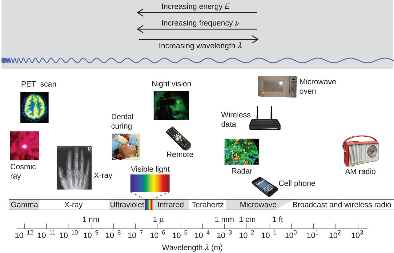
Different parts of the electromagnetic spectrum typically use different units: Low-energy photons, such as microwaves and radio waves, are specified in frequencies (MHz or GHz); mid-energy photons, such as infrared and visible light, are specified in wavelengths (μm, nm, pm, or Å); high-energy photons, such as x-rays and gamma-rays, are specified in energies (keV or MeV).
Our eyes detect visible-range photons, allowing us to see the world around us. But scientific instruments allow us to “see” lots more by detecting photons over a much wider range of energies. For example, studies of atomic spectra, experiments involving interaction of gaseous matter with visible, ultraviolet, and infrared light, led to better understanding of the structure of atoms.
D2.2 Atomic Spectra
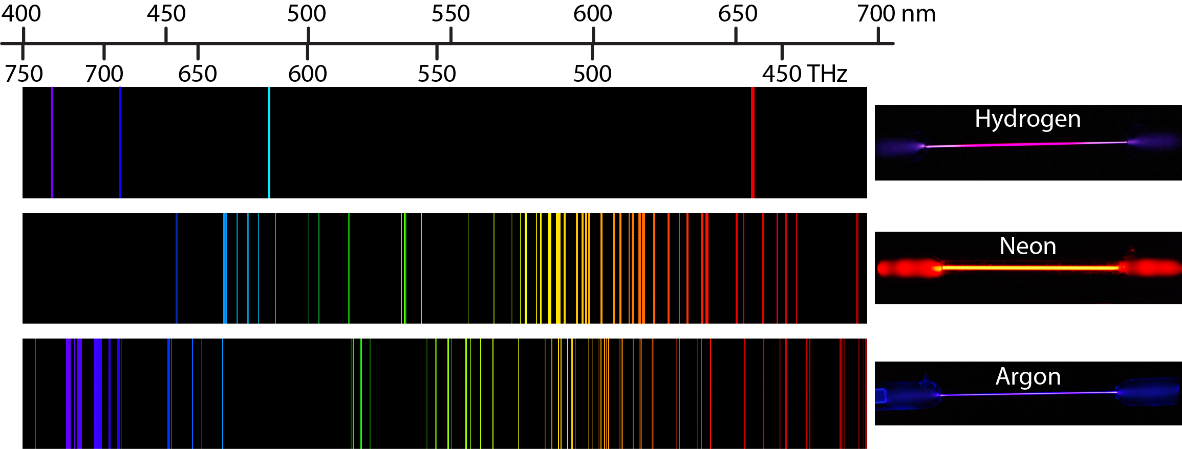
Heating a gaseous element at low pressure or passing an electric current through the gas imparts additional energy into the atoms. These higher energy atoms can then release the additional energy by emitting photons. For instance, the colors of “neon” signs are produced by passing electric current through low-pressure gases. Interestingly, the photons emitted by the higher-energy atoms have only a few specific energies, thereby producing a line spectrum consisting of very sharp peaks (lines) at a few specific frequencies. Line spectra were intriguing because there was no reason to expect that some frequencies would be preferred over others.
Each element displays its own characteristic set of lines. For example, when electricity passes through a tube containing H2 gas at low pressure, the H2 molecules are broken apart into separate H atoms and the H atoms emit a purple color. Passing the purple light through a prism produces the uppermost line spectrum shown in Figure 2: the purple color consists of four discrete visible wavelengths: 656.4 nm, 486.2 nm, 434.1 nm, and 410.2 nm.
The H-atom emission spectrum also contains lines in the ultraviolet and infrared ranges. In 1888, Johannes Rydberg developed an equation that predicts wavelengths for all hydrogen emission lines:
Here, n1 and n2 are positive integers with n2 < n1, and the Rydberg constant R∞ = 1.09737316 × 10⁷ m−1.
Because the wavelengths of hydrogen emission lines were measured to very high accuracy, the Rydberg constant could be determined very precisely. That a simple formula involving integers could account for such precise measurements seemed astounding at the time.
Exercise 2: Hydrogen-Atom Emission
Use the Rydberg equation to calculate the wavelength of the photon emitted by a hydrogen atom when n2 = 3 and n1 = 7.
D2.3 Atomic Energy Levels
Why should a hydrogen atom emit only four specific colors of visible light? To understand this better, we need to know more about the energy of the atom and how energy depends on atomic structure. Any atom consists of a tiny nucleus surrounded by one or more electrons. The simplest atom, a hydrogen atom, has one proton as the nucleus and one electron outside the nucleus. According to Coulomb’s law, the electron and proton attract.
Exercise 3: Electrostatic Potential Energy
Activity 2: Line Spectra and Energies
The model currently used to describe the distribution of electrons in an atom has these attributes:
- The energies of electrons in an atom are restricted to energy levels, which are specific allowed energies.
- Each line in the spectrum of an element results when an electron’s energy changes from one energy level to another; a change from one electronic energy level to another is called an electronic transition.
- Electrons are distributed in regions centered on the nucleus, called shells; each shell has a different average distance from the nucleus.
- As described by Coulomb’s law, an electron’s energy increases with increasing average distance from the nucleus; that is, with increasing size of an electron shell.
- Both energy levels and shells are described by quantum numbers, numbers restricted to specific allowed values; the electron energies are said to be quantized, restricted to discrete energy levels.
An atom is most stable when it has the lowest possible energy. The lowest energy electronic state of an atom is called its electronic ground state (or simply ground state). Any higher energy state of an atom is called an electronic excited state (or simply an excited state).
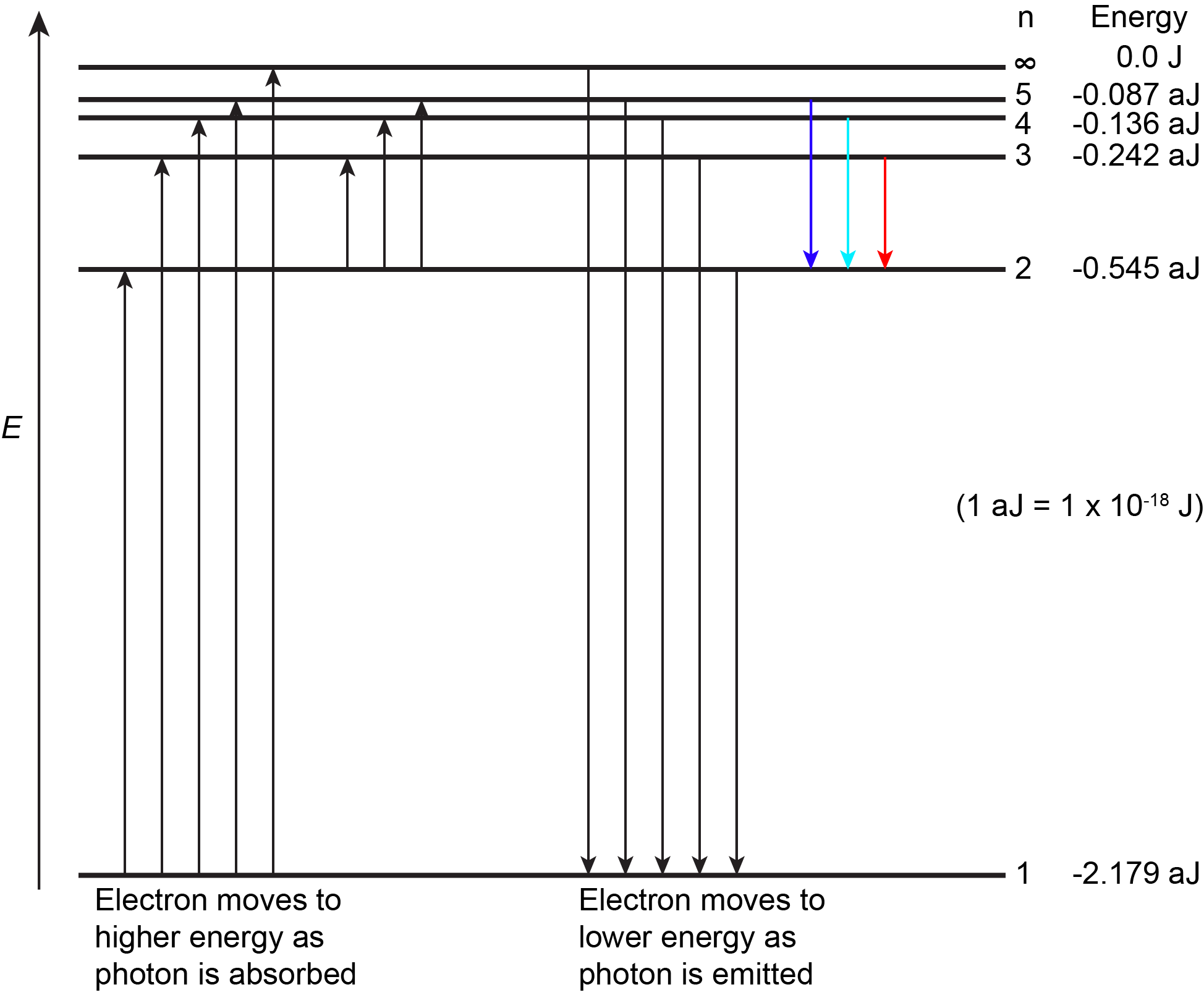
Figure 3 shows the first few energy levels of a hydrogen atom. The atom is in its ground state when its electron is in the n = 1 (lowest energy) level. When a photon is absorbed by a ground state hydrogen atom, as shown on the left side of Figure 3, the energy of the photon moves the electron to a higher n (higher energy) level, and the atom is now in an excited state.
An atom in an excited state can release the extra energy as a single photon if the electron returns to its ground state (say, from n = 5 to n = 1), or the energy can be released as two or more lower energy photons if the electron falls to an intermediate state then to the ground state (say, from n = 5 to n = 2, emitting one photon, then from n = 2 to n = 1, emitting a second photon).
D2.4 The Quantum Mechanical Model of the Hydrogen Atom
If we could calculate the energy for each energy level, we could predict the emission spectrum for hydrogen. In 1926, Erwin Schrödinger applied quantum mechanics, a model that uses both wave and particle analogies to describe atomic-scale matter, to the hydrogen atom. Instead of viewing the electron as a particle, Schrödinger applied mathematics appropriate for three-dimensional stationary waves constrained by electrostatic potential (Coulomb’s-law attraction between electron and nucleus). For each wave he derived a mathematical function to describe the wave, a wave function. The wave function is typically designated by the Greek letter ψ.
Schrödinger showed that these wave functions could be used to calculate allowed energies of a hydrogen atom. The calculated energies are given by this equation:
\[{E_{\rm{n}}} =\ – \frac{k}{{{n^2}}},{\rm{\ \ }}n = 1,2,3, \ldots \]
where the proportionality constant k = 2.179 × 10⁻¹⁸ J, and n is a quantum number restricted to positive integer values.
In an electronic transition, an electron moves from one energy level to a different energy level. The energy of the corresponding photon is the energy difference between the two energy levels, an initial level with energy Ei and a final level with energy Ef.
[latex]{\rm{\Delta }}E = {E_{\rm{f}}} - {E_{\rm{i}}} = - k\left( {\dfrac{1}{{n_{\rm{f}}^2}} - \dfrac{1}{{n_{\rm{i}}^2}}} \right)[/latex]
A positive ΔE means that the atom’s energy increased, corresponding to absorption of a photon: the photon’s energy has been added to the atom’s initial energy. Similarly, a negative ΔE means that the atom has lost energy through emission of a photon.
Conservation of energy requires that the energy of the photon, Ephoton = hc/λ, equals the absolute value of the energy difference, |ΔE|, for emission or absorption. The sign of ΔE indicates whether the photon was absorbed (+) or emitted (−).
Exercise 4: Hydrogen-Atom Electronic Transition Energy
The equation Schrödinger obtained is equivalent to the equation Rydberg used to calculate hydrogen emission lines:
\[{E_{{\rm{photon}}}} = \frac{{hc}}{\lambda } = {\rm{|\Delta }}E| = \left| { – k\left( {\frac{1}{{n_{\rm{f}}^2}} – \frac{1}{{n_{\rm{i}}^2}}} \right)} \right|\]
\[\frac{1}{\lambda } = \frac{k}{{hc}}\left( {\frac{1}{{n_{\rm{f}}^2}} – \frac{1}{{n_{\rm{i}}^2}}} \right) = {R_\infty }\left( {\frac{1}{{n_{\rm{2}}^2}} – \frac{1}{{n_{\rm{1}}^2}}} \right)\]
and thus, R∞ = k/(hc). Substituting values for k, h, and c into this equation gives R∞ = 1.097× 10⁷ m−1, which is the same as the experimental Rydberg constant to four significant figures. That a wave model could reproduce these highly accurate energy levels was strong evidence that quantum mechanics is an appropriate atomic-level model.
D2.5 Wave-Particle Duality
The combined wave and particle model is referred to as wave-particle duality. Its impact in describing atomic-scale particles (protons and electrons) is dramatic: wave-particle duality implies that we should not just think of an electron as located at a specific position around a nucleus or moving in a specific direction and with a specific speed: the wave-like electron seems to be all around the nucleus at once! In other words, the wave nature of an electron is just as important in describing its properties as its particle nature.
An important consequence of wave-particle duality is the Heisenberg uncertainty principle: it is impossible to determine the exact position and the exact momentum of an atomic-level particle simultaneously. This means that, if we know exactly where an electron is at one instant, we have no idea where it will be an instant later; or, if we know an electron’s exact speed and direction, we have no information about where it is. As a result of the uncertainty principle, the best we can do is determine the probability of finding an electron at a specific position; that probability is proportional to the square of the wave function, ψ2.
The electron-density distribution (or just electron density) is the three-dimensional distribution of electron probability, which can be derived from the square of a wave function. Wave functions and their electron-density distributions are called orbitals. It is these orbitals that help us understand atomic properties, chemical bonds, and forces between molecules.
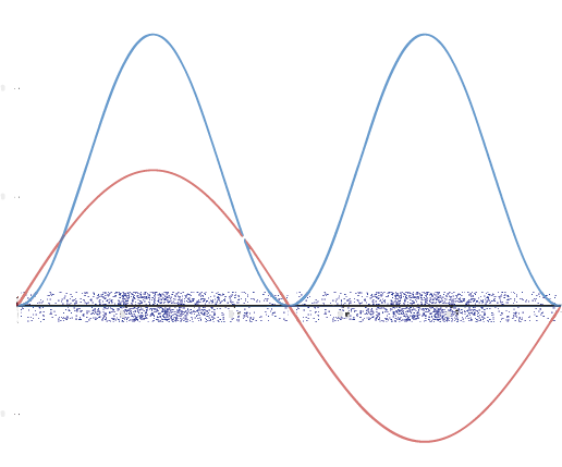
A graphic way of showing electron-density distribution (depicting an orbital) is by the density of shading or stippling. That is, we draw lots of dots or darker shading where the probability is high and we draw fewer dots where the probability is low. For example, consider the wave shown below in red along with its square shown in blue. Wherever there is a maximum in the square of the wave function (blue curve), there are many dots. Where the wave function (and therefore also its square) approaches zero, there are few dots.
Such a way to visualize electron density is quite useful for a 3-D view of the electron density surrounding a nucleus. For example, you can see the electron-density distribution of a hydrogen atom in its ground state in this video, where the hydrogen atom is rotated around its nucleus.
In your class notebook write a description of (1) the shape of the electron density distribution for a ground-state H atom and (2) how electron density changes with distance from the nucleus. (The nucleus is located at the intersection of the three axes: x, y, and z axes).
In the electron-density diagram below, click on the white cross that corresponds to the lowest electron density.
Based on the density of dots in the diagram, make a graph with electron density on the vertical axis and distance from the nucleus on the horizontal axis. How is a graph of wave function versus distance from the nucleus related to the graph you made?
Similar to dot-density diagrams, but visually simpler while conveying a little less information, are 3-D boundary-surface plots, which show a surface that has the same shape as the electron density distribution and encloses some fraction, such as 90%, of the electron density. That is, if we could repeatedly locate the electron exactly, nine times out of ten the electron would be located inside the boundary surface. The figure below shows how a boundary surface is related to the dot-density plot you have already viewed. Move the slider at the bottom to change from dot-density to boundary-surface diagram.
Visualizing electron-density distributions confirms an idea mentioned earlier: there are shells of electron density, concentric spheres each farther from the nucleus. The orbitals that belong to a given shell have the same quantum number, n and their electron density is approximately the same average distance from the nucleus. The principal quantum number n dictates the overall size of the orbital.
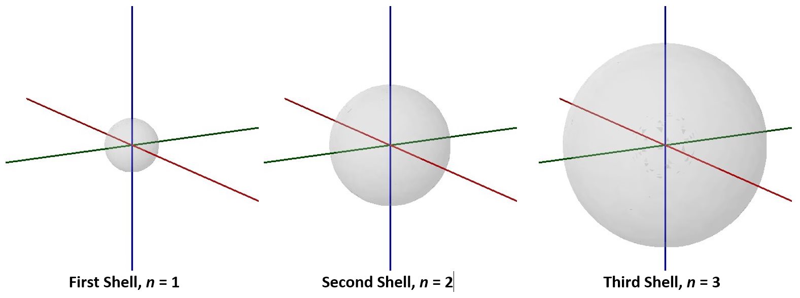
As n gets larger, the radius, r, of the electron shell gets larger, and En becomes less negative—closer to zero. Therefore, the limits n ⟶ ∞ and r ⟶ ∞ imply that En = 0 corresponds to ionization of the atom, complete separation of the electron from the nucleus. Thus, for a hydrogen atom in the ground state, the ionization energy is:
Another interesting aspect is that while we know En, which is the total energy of the electron, we cannot measure the electron’s kinetic energy (or its velocity) and potential energy separately. We know from Coulomb’s law that the potential energy changes as a function of r. Since the electron density is distributed over a range of r, there’s a range of potential energy, and hence a range of kinetic energy—when the electron’s potential energy is higher, its kinetic energy would be lower. This uncertainty is again related to the wave nature of the electron. However, knowing the total energy, En, is quite sufficient for us!
Activity 4: Wrap-up—Atomic Spectra and Atomic Structure
D2.6 Atomic Orbitals and Quantum Numbers
Quantum Numbers: n, ℓ, mℓ
The atomic wave functions can be defined using three quantum numbers: n, ℓ, and mℓ. Each wave function corresponds to an atomic orbital. Each atomic orbital defines a region in the atom within which electron probability density is large.
The energy of a hydrogen atom orbital depends on the principal quantum number, n:
As discussed above, the size of the orbital (the average distance of the electron from the nucleus) increases as n increases. The farther the electron is from the nucleus, the higher (less negative) the energy is.
The second quantum number, ℓ, is the orbital quantum number (sometimes called azimuth or angular-momentum quantum number). It determines the shape of the electron-density distribution. ℓ is an integer with values ranging from 0 to n – 1; that is, ℓ = 0, 1, 2, …, n – 1. Thus, an orbital with n = 1 can have only one value of ℓ, ℓ = 0, whereas n = 2 permits ℓ = 0 and ℓ = 1, and so on.
Values of ℓ are designated using letters:
| ℓ = 0 | s orbitals |
| ℓ = 1 | p orbitals |
| ℓ = 2 | d orbitals |
| ℓ = 3 | f orbitals |
| ℓ = 4 | g orbitals |
| ℓ = 5 | h orbitals |
View the shapes of s, p, and d orbitals shown in these videos:
1s orbital 2p orbital 3d orbital
In your class notebook write a description of the shape of the electron density distribution for each orbital. Also, make a rough drawing of the corresponding boundary-surface diagram for each dot-density diagram.
The magnetic quantum number, mℓ, specifies the spatial orientation of a particular orbital. Values of mℓ can be any integer from –ℓ to ℓ. For example, for an s orbital, ℓ = 0, and the only value of mℓ is 0; thus there is only a single s orbital. For p orbitals, ℓ = 1, and mℓ can be equal to –1, 0, or +1; thus there are three different p orbitals, which are commonly shown as px, py, and pz, oriented along the x, y, and z axes.
The total number of possible orbitals with the same value of ℓ is 2ℓ + 1. There are five d orbitals, seven f orbitals, and so forth. The sizes and shapes of s, p, and d orbitals in the first three shells are shown in Figure 6. Each of these orbitals corresponds to a different set of n, ℓ, and mℓ values.
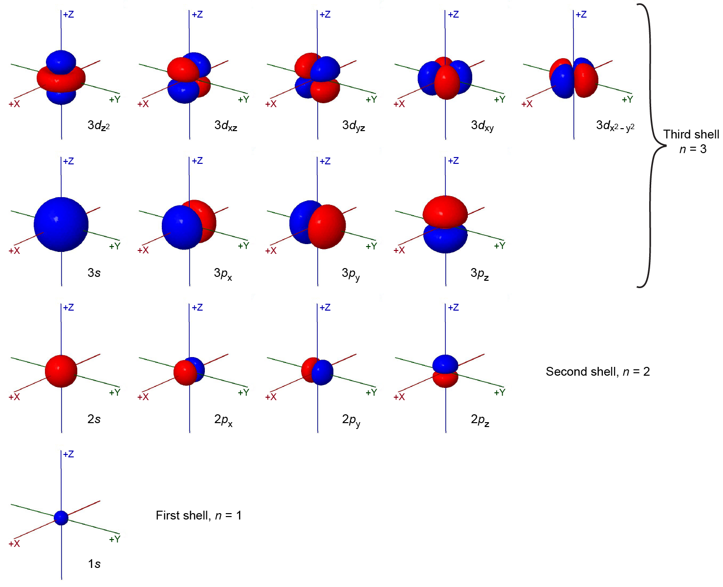
All orbitals with the same value of n and ℓ form a subshell. For example, the 2px, 2py, and 2pz orbitals constitute the 2p subshell because each of these orbitals has n = 2 and ℓ = 1. The number of orbitals in a subshell equals the number of different values for the mℓ quantum number. Each shell contains n subshells: for example, when n = 3, there is a 3s, a 3p, and a 3d subshell, corresponding to the three possible ℓ values of 0, 1 and 2.
Orbital Phases and Nodes
Figure 6 shows some atomic orbitals as either all blue or all red (for example, 1s and 2s), while other orbitals contain both colors (for example, the 2p orbitals). The blue and red colors show the mathematical sign of the wave function, a property called the phase of the wave function. Most wave functions are positive in some regions and negative in others. Phase is important when wave functions on two atoms interact to form a chemical bond.
The relationship between wave function and electron density is depicted more explicitly in Figure 7. In the middle row, boundary-surface diagrams from Figure 6 show the sizes and shapes of electron-density distributions for the 1s, 2s, and one of the 2p orbitals. In the top row are the corresponding wave functions (ψ); the bottom row shows electron density, ψ2.
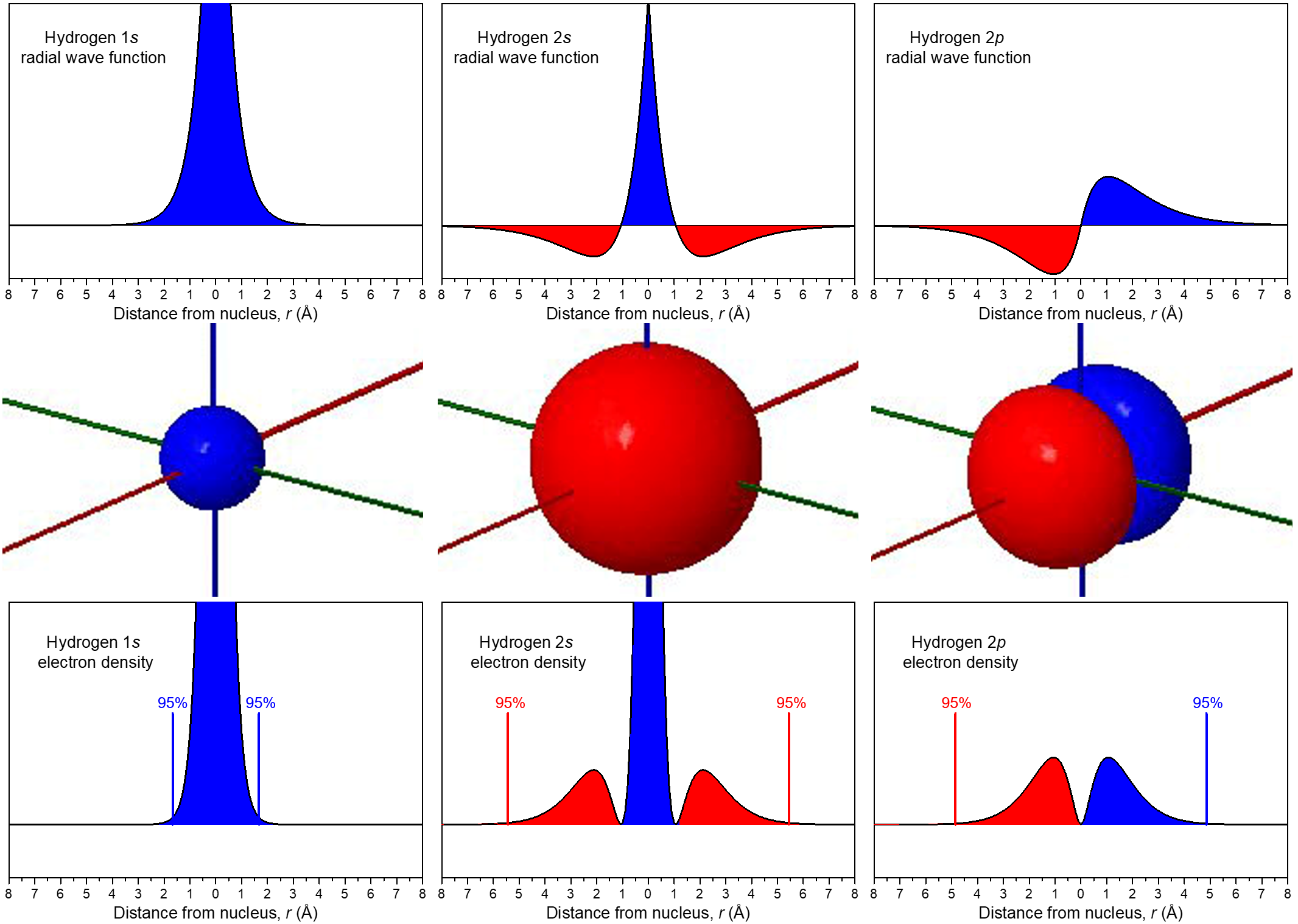
The wave functions and electron-density functions are color coded to show the regions where ψ > 0 as blue and the areas where ψ < 0 as red. A surface where the wave function changes sign is called a node. At a node, ψ = 0 and therefore the probability of finding the electron in that surface is also 0.
For the 1s orbital, there are no nodes; its wave function only has positive values. For the 2s orbital, there is one node at r = 1.05 Å; the wave function goes from positive values near the nucleus to negative values farther out. (You cannot see this node in the boundary-surface diagram, because the node is a sphere that is within the volume enclosed by the boundary surface.) A node that occurs at a specific value of r is a radial node, and therefore radial nodes have a spherical shape. The 3s orbital, for example, has two radial nodes enclosed within the boundary-surface diagram.
Each 2p orbital has one node. Look at the boundary-surface diagram to verify that this node is planar instead of spherical. Non-spherical nodes are angular nodes. For example, the 2px orbital has one angular node: the yz plane; ψ is equal to 0 at all points in the yz plane, rather than at any specific r value. You can see the presence of angular nodes clearly in boundary-surface diagrams.
An orbital has n – 1 nodes, of these, n – 1 – ℓ are radial nodes, and the number of angular nodes corresponds to the value of ℓ. A generalization that is true for all kinds of waves is that the greater the total number of nodes, the higher the energy. The phase of the wave function differs on either side of a node, because the wave function changes from one mathematical sign to the other as it crosses a node. Visually, we represent these different phases, and the presence of nodes, with different colors in the boundary-surface diagram.
Fourth Quantum Number, ms
The fourth quantum number, called the spin quantum number, ms, differs from the other three quantum numbers in that it describes the electron rather than the orbital. An electron has a very small magnetic field. Moving a macroscopic charge in a circular path produces a magnetic field, so initially the electron’s magnetic field was attributed to its spinning like a top; hence the name “spin quantum number”. The electron’s magnetic field can have two quantized states: either “up” or “down”. This gives two possible ms values, ms = +½ or ms = -½. When an electron occupies an orbital, we typically depict these two possible ms values as an ↑ or ↓ arrow.
In your class notebook make a table summarizing the names, symbols, allowed values, and important properties of the four quantum numbers. (You can use this table for studying later.) If you are studying with someone else, make your tables independently and then compare.
When you are satisfied with your table, compare it with ours.
This Podia problem is based on today’s pre-class material; working through that material will help you solve the problem.
Consider these two sentences: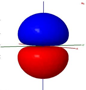
- The surface shown in this illustration of an atomic orbital is chosen so that the entirety of the electron’s wave function is enclosed.
- The colors in the diagram represent regions of opposite electron spin.
Decide whether each sentence is correct. Rewrite all incorrect text so that it is correct. Be brief but include all important ideas and use scientifically appropriate language.
Two days before the next whole-class session, this Podia question will become live on Podia, where you can submit your answer.
