
Unit Four
Day 30: ICE Table, Reaction Quotient, Le Châtelier’s Principle
D30.1 ICE Table
An ICE table (for Initial concentration, Change in concentration, and Equilibrium concentration) is a good methodology for calculating an equilibrium constant from experimental data. ICE tables also help to solve many other types of equilibrium problems.
An ICE table begins with the balanced reaction equation, using the reactants and products as column headings. The second row lists the initial concentrations of the reactants and products; these can usually be obtained from experimental data based on the assumption that no reaction has yet taken place. The third row is the change in concentration that occurs as the system proceeds toward equilibrium; this row is derived from the stoichiometry of the reaction. The last row is the sum of the first two rows, which yields the equilibrium concentrations.
For example, consider determining the equilibrium constant for the reaction:
If a solution initially has [I2]0 = [I−]0 = 1.000 × 10⁻³ M and no triiodide ions ([I3−] = 0), and then reacts to give an equilibrium concentration of [I2]e = 6.61 × 10⁻⁴ M, we can use an ICE table to determine the equilibrium constant for the reaction. First, write the balanced reaction at the top of the table. The next row gives the initial concentrations.
| I2(aq) | + | I‾(aq) | ⇋ | I3‾(aq) | |
| Initial concentration (M) | 1.000 × 10⁻³ | 1.000 × 10⁻³ | 0 | ||
| Change in concentration (M) | –x | –x | +x | ||
| Equilibrium concentration (M) | (1.000 × 10⁻³) – x | (1.000 × 10⁻³) – x | x |
In the “Change” row, the mathematical sign indicates the direction of change: the sign is positive when the concentration increases as the reaction proceeds toward equilibrium, and negative when the concentration decreases. For example, because the reaction starts with no I3‾, [I2]t must decrease as the reaction proceeds, so its (unknown) change in concentration is “-x“. In general, x is also multiplied by the stoichiometric coefficient, but in this case, all coefficients are 1, so that is not obvious.
Using the information that [I2]e = 6.61 × 10⁻⁴ M, we can solve for x:
| (1.000 × 10⁻³) – x | = | 6.61 × 10⁻⁴ M |
| x | = | 3.39 × 10⁻⁴ M |
and then calculate the equilibrium constant Kc:
Exercise 1: Concentration Changes During Reactions
Activity 1: Calculating Equilibrium Concentrations I
Activity 2: Calculating Equilibrium Concentrations II
D30.2 “All-Reactant” or “All-Product” Starting Point
The same equilibrium concentrations are achieved whether a reaction begins with only reactants present or only products present. Let’s use an example to consider this in further detail. HF is a deadly, but weak, acid. It ionizes partially in water :
What are the equilibrium concentrations of the various aqueous species in a solution of 0.150-M HF?
One way to determine these equilibrium concentrations is to start with only reactants. This is called the “all-reactant” starting point.
Activity 3: All-reactant Starting Point
Alternatively, we could solve the problem assuming that all the HF ionizes first, and then the system comes to equilibrium. This is called the “all-product” starting point.
Activity 4: All-product Starting Point
The two approaches give the same results, and show that starting with all products leads to the same equilibrium conditions as starting with all reactants. Note that this is true only if the temperature is the same and the same total number of atoms of each kind is present in both cases. Here we either started with all reactants, 0.150-M HF (which contains 0.150 mol/L H and 0.150 mol/L F), or with all products, 0.150–M H+ and 0.150-M F− (which also contains 0.150 mol/L H and 0.150 mol/L F). Had we started with 0.140-M H+ and 0.160-M F−, the equilibrium concentrations would not be the same.
For the ionization of HF(aq) the equilibrium constant is small: Kc = 6.80 × 10⁻⁴. That is, the ionization of HF(aq) is reactant-favored. In Activity 3 the change in concentration, x3 = 0.00977, while in Activity 4 the change in concentration, x4 = 0.140. Because the process is reactant-favored, the all-reactant initial concentrations are much closer to the equilibrium concentrations than the all-product initial concentrations. Therefore the all-reactants situation involves only small changes in concentrations to reach equilibrium. Recognizing this allows making approximations that can significantly simplify the calculations in equilibrium problems.
We know that when Kc << 1, the equilibrium is significantly reactant-favored, and when Kc >> 1, the equilibrium is significantly product-favored. If the ICE table can be set up so that the “initial” concentrations are close to equilibrium (either all-reactant or all-product, depending on the size of Kc), then any change in concentration that is small compared to the initial concentrations can be neglected. “Small” is defined as resulting in an error that does not change the answer within the the number of significant figures involved.
Activity 5: Solving an Aqueous Equilibrium Problem
D30.3 Reaction Quotient
Starting with only reactants present means that the reaction must initially be spontaneous left to right, even if only very small concentrations of products are present when equilibrium is reached. Starting with only products present requires that the reaction go from right to left. Which direction does a reaction go when both reactants and products are present but the reaction is not at equilibrium? The reaction quotient can answer this question.
For a generic reaction,
the reaction quotient (Q) is defined as:
In Qc the subscript “c” indicates Q is in terms of concentrations; for a gas-phase reaction we could write Qp similarly in terms of partial pressures.
The concentrations are represented by “[…]t” to emphasize that Qc for a reaction depends on the concentrations present at the time when Qc is determined; this is usually not at equilibrium. When only reactants are present, Qc = 0. As the reaction proceeds, Qc increases because product concentrations increase and reactant concentrations decrease (Figure 1). When the reaction reaches equilibrium, Qc no longer changes over time because the concentrations no longer change, and, at equilibrium, Qc = Kc:
![Four graphs are shown. The y-axis on top left graph is labeled, “Concentration,” and the x-axis is labeled, “Time.” Three curves are plotted on graph. The first is labeled, “[ S O subscript 2 ];” this line starts high on the y-axis, ends midway down the y-axis, has a steep initial slope and a more gradual slope as it approaches the far right on the x-axis. The second curve on this graph is labeled, “[ O subscript 2 ];” this line mimics the first except that it starts and ends about fifty percent lower on the y-axis. The third curve is the inverse of the first in shape and is labeled, “[ S O subscript 3 ].” The y-axis on top right graph is labeled, “Concentration,” and the x-axis is labeled, “Time.” Three curves are plotted on graph b. The first is labeled, “[ S O subscript 2 ];” this line starts low on the y-axis, ends midway up the y-axis, has a steep initial slope and a more gradual slope as it approaches the far right on the x-axis. The second curve on this graph is labeled, “[ O subscript 2 ];” this line mimics the first except that it ends about fifty percent lower on the y-axis. The third curve is the inverse of the first in shape and is labeled, “[ S O subscript 3 ].” The y-axis on bottom left graph is labeled, “Reaction Quotient,” and the x-axis is labeled, “Time.” A single curve is plotted on graph c. This curve begins at the bottom of the y-axis and rises steeply up near the top of the y-axis, then levels off into a horizontal line. The top point of this line is labeled, “kc.”](https://wisc.pb.unizin.org/app/uploads/sites/461/2019/04/Qc_SO3.png)
A system that is not at equilibrium proceeds spontaneously in the direction that establishes equilibrium (Qc changes until it equals Kc). Hence, we can predict directional shifts of a reaction by comparing Qc to Kc: when Qc < Kc, the reaction proceeds spontaneously from left to right (to the product side); when Qc > Kc, the reaction proceeds spontaneously to the left (reactant side).
For example, for the water-gas shift reaction,
different starting mixtures of CO, H2O, CO2, and H2 react (and the concentrations of reactants and products change) until the compositions reach the same value of Qc; that is, until Qc = Kc (Figure 2).
It is important to recognize that Qc reaches the same equilibrium value (Kc) whether the reaction starts from all reactants, from all products, or from a mixture of both. In fact, one technique to determine whether a reaction is truly at equilibrium is to start with only reactants in one experiment and start with only products in another. If the same value of the reaction quotient is observed when the concentrations have stopped changing in both experiments, then it is highly likely that the system has reached equilibrium.
Exercise 2: Determining Which Direction a Reaction Goes
D30.4 Le Châtelier’s principle: Change in Concentration
Le Châtelier’s principle states that when a chemical system is at equilibrium and conditions are changed so that the reaction quotient, Q, changes, the chemical system will react to achieve new equilibrium concentrations or partial pressures; reaction occurs in a way that partially counteracts the change in conditions. To establish the new equilibrium, the reaction proceeds in the forward direction if Q < K or in the reverse direction if Q > K, until Q is again equal to K.
For a chemical system at equilibrium at constant temperature, if the concentration of a reactant or a product is changed, therefore changing Q, the system is no longer at equilibrium because Q ≠ K. The concentrations of all reaction species will then undergo additional changes until the system reaches a new equilibrium with a different set of equilibrium concentrations. We say that the equilibrium shifts in a direction (forward or reverse) that partially counteracts the change.
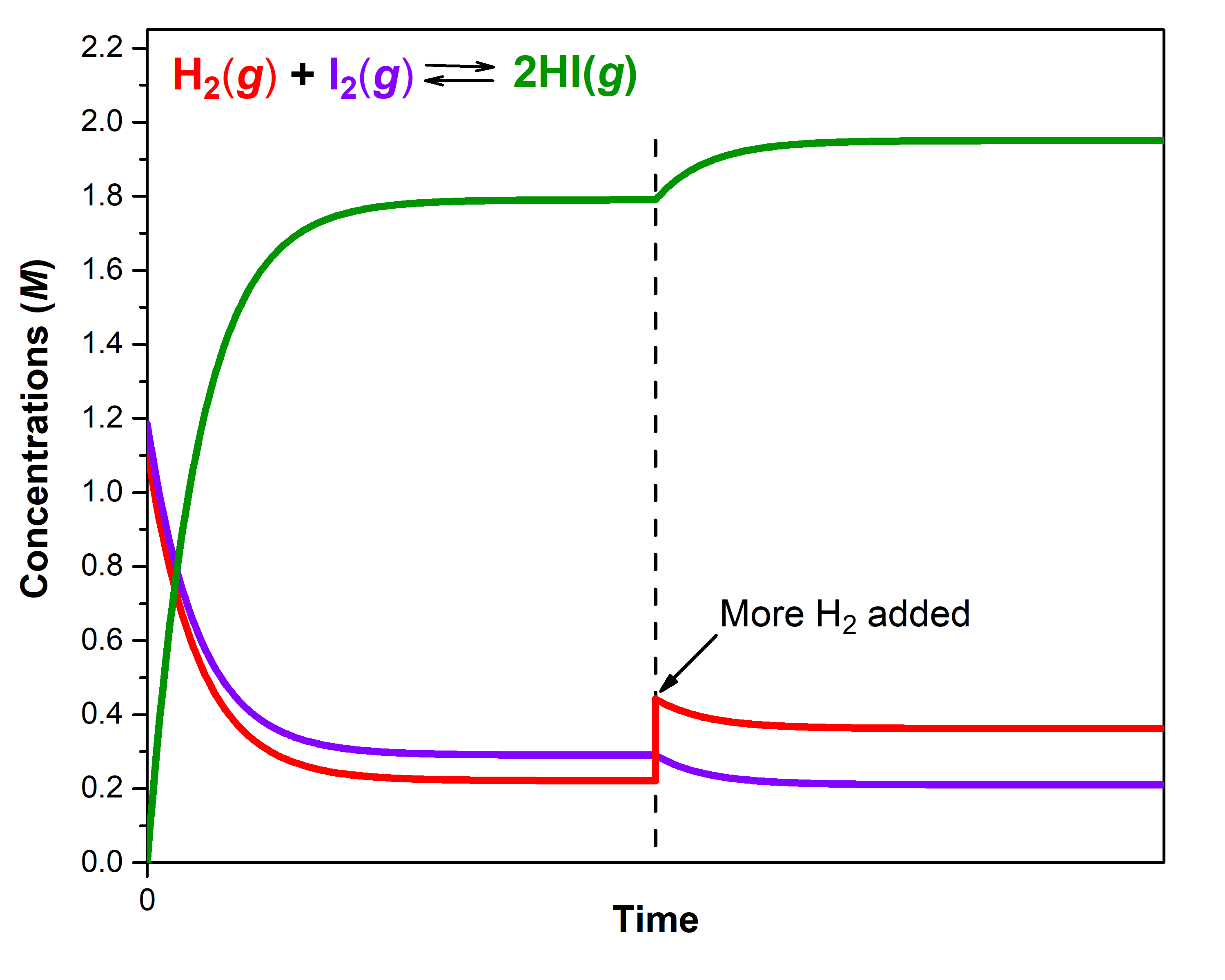
For example, consider the chemical reaction:
A mixture of gases at 400 °C with [H2]e1 = 0.221 M, [I2]e1 = 0.290 M, and [HI]e1 = 1.790 M is at equilibrium in a closed container. For this mixture, Qc = Kc = 50.0. If additional H2 is introduced into the container quickly such that [H2] doubles before it begins to react (that is, the new [H2]t = 0.442 M), Qc is now ½ of Kc:
The reaction then proceeds in the forward direction to reach a new equilibrium. Experimental measurements show that at the new equilibrium [H2]e2 = 0.362 M, [I2]e2 = 0.210 M, and [HI]e2 = 1.950 M. Notice that [H2]e2 (0.362 M) is less than the doubled concentration (0.442 M) but more than [H2]e1 (0.221 M). The equilibrium has shifted to partially counteract the change in H2 concentration. Because of the shift, the concentration of the other reactant decreases and the concentration of the product increases. To verify that these new concentrations are equilibrium concentrations, calculate Q:
Another way to think about the shift in equilibrium is to recall that at equilibrium, rateforward = ratereverse. The forward reaction is first-order in H2, so doubling the concentration of H2 doubles rateforward, making rateforward > ratereverse. As the equilibrium shifts, the concentrations of both reactants decrease and the concentration of product increases until new equilibrium concentrations are reached, where forward and reverse reactions have reached new, but equal, rates.
Figure 3 illustrates graphically the effect of adding H2 to the reaction at equilibrium.
D30.5 Le Châtelier’s Principle: Change in Pressure or Volume
Changes in pressure have a measurable effect on equilibrium in systems involving gases if the chemical reaction produces a change in the total number of gas molecules (that is, if the number of gas molecules on the reactant side differs from the product side). The overall change in pressure must affect partial pressures of reactants and/or products: adding an inert gas that is not a reactant or product changes the total pressure but not the partial pressures of the gases in the equilibrium constant expression, and therefore does not perturb the equilibrium.
Consider what happens when the volume decreases for this equilibrium:
Decreasing the volume increases the total pressure and increases the partial pressure of each gas. The equilibrium shifts to partially counteract the increase in pressure. Formation of additional NO2 decreases the total number of gaseous molecules in the system because each time two molecules of NO2 form, a total of three molecules of NO and O2 react away. This reduces the total pressure exerted by the system and partially counteracts increased pressure. LeChatelier’s principle predicts that the equilibrium shifts to the right, toward products.
We can also look at this by considering Qc. Reducing the system volume increases the partial pressure (or concentration) of all gaseous species. If the volume is reduced by half, then each partial pressure becomes twice what it was for the previous equilibrium:
Because Qc < Kc, the reaction proceeds toward the product side (forming additional NO2) to re-establish equilibrium.
Now consider this reaction:
Because there is no change in the total number of gaseous molecules in the system during reaction, a change in pressure does not shift the equilibrium towards either reactant or product side.
For reactions in solution, changing the solution volume changes the concentrations of all reaction species. Therefore, when solvent is added (the solution is diluted), the equilibrium shifts toward the side with more solute particles, partially compensating for the dilution of total concentration. If solvent is removed (by evaporation, for example) so that all solute concentrations increase, the equilibrium shifts toward the side with fewer solute particles, decreasing the total concentration of solute particles.
For example, when enough water is added to this equilibrium to double the solution volume:
the concentration of each solute is halved compared to the initial equilibrium concentration. Hence:
Because Qc > Kc the reaction proceeds toward the reactant side (the side with more solute particles) as equilibrium is re-established.
Exercise 3: Using Le Chatelier’s Principle at Constant Temperature
Podia Question
This question explores Le Chatelier’s principle applied to the equilibrium between hydrogen, nitrogen, and ammonia:
N2(g) + 3 H2(g) ⇌ 2 NH3(g) Kp = 5.8 × 10⁶ atm−2 at 25 °C
a) Write the expression for Kp for this reaction.
b) Predict the effect on the equilibrium (at 25 °C) of an increase in each partial pressure:
i) PN2
ii) PH2
c) Suppose that 0.245 mol N2, 0.00145 mol H2, and 0.162 mol NH3 occupy a 10.0-L volume; the partial pressures are PN2= 0.600 atm, PH2= 0.00356 atm, and PNH3= 0.396 atm and the total pressure is 1.00 atm. Is the system at equilibrium? If not, in which direction would the reaction shift to reach equilibrium? Show a calculation to support your answer.
d) Suppose the total pressure is kept constant and that 0.010 mol N2 is added to the system described in part c so that the total amount of N2 is 0.255 mol and the total amount of all gases is 0.418 mol. If the total pressure stays constant, what must happen to the volume? Why?
e) Based on the ideal gas law it is possible to calculate the new volume of the mixture of gases and to calculate the partial pressures of the constituent gases. The partial pressures are PN2 = 0.610 atm, PH2 = 0.00347 atm, and PNH3 = 0.388 atm. Is the system at equilibrium? If not, in which direction does the reaction shift to reach equilibrium? Show a calculation to support your answer.
f) Does your answer in part (e) agree with your first answer in part b? Explain why or why not.
g) Have you discovered an exception to Le Chatelier’s principle? Explain why or why not.
Two days before the next whole-class session, this Podia question will become live on Podia, where you can submit your answer.
