
Additional Reading Materials
Chapter 12: Entropy and Gibbs Free Energy
Ch12.1 Entropy
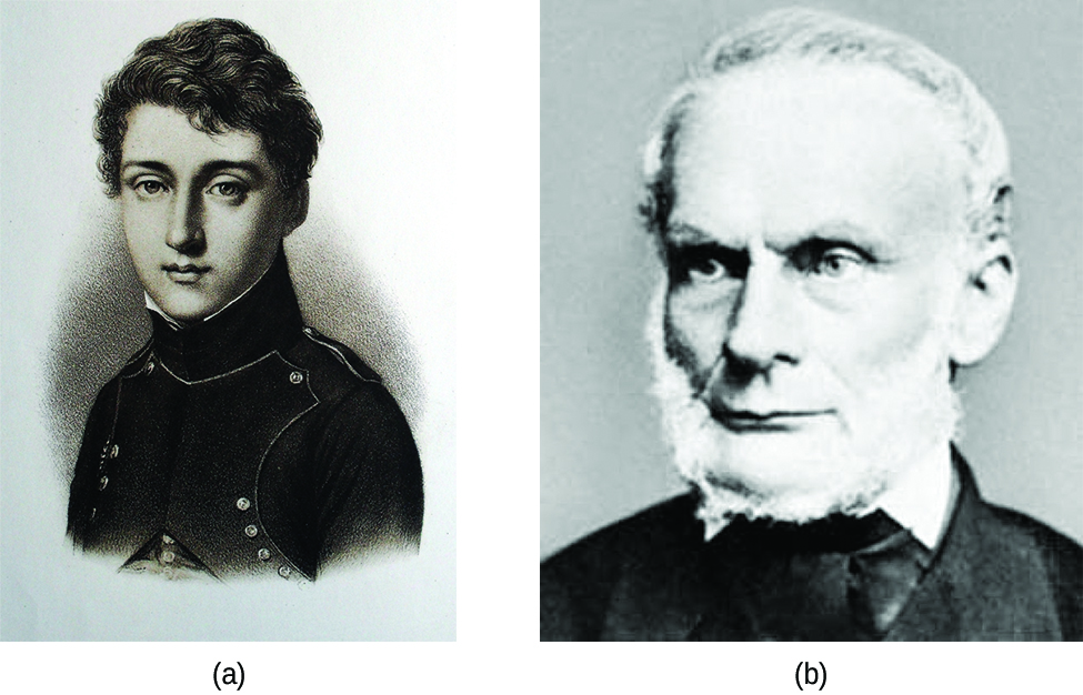
In 1824, at the age of 28, Nicolas Léonard Sadi Carnot (Figure 1) published the results of an extensive study regarding the efficiency of steam heat engines. In a later review of Carnot’s findings, Rudolf Clausius introduced a new thermodynamic property that relates the spontaneous heat flow accompanying a process to the temperature at which the process takes place. This new property was expressed as the ratio of the reversible heat (qrev) and the kelvin temperature (T). The term reversible process refers to a process that takes place at such a slow rate that it is always at equilibrium and its direction can be changed (it can be “reversed”) by an infinitesimally small change in some condition. Note that the idea of a reversible process is a formalism required to support the development of various thermodynamic concepts; no real processes are truly reversible, rather they are classified as irreversible.
Similar to other thermodynamic properties, this new quantity is a state function, and so its change depends only upon the initial and final states of a system. In 1865, Clausius named this property entropy (S) and defined its change for any process as the following:
The entropy change for a real, irreversible process is then equal to that for the theoretical reversible process that involves the same initial and final states.
Ch12.2 Entropy and Microstates
Following the work of Carnot and Clausius, Ludwig Boltzmann developed a molecular-scale statistical model that related the entropy of a system to the number of microstates possible for the system. A microstate (W) is a specific configuration of the locations and energies of the atoms or molecules that comprise a system:
Here k is the Boltzmann constant and has a value of 1.38 × 10⁻²³ J/K.
The change in entropy for a process is the difference between its final (Sf) and initial (Si) values:
For processes involving an increase in the number of microstates, Wf > Wi, the entropy of the system increases, ΔS > 0. Conversely, processes that reduce the number of microstates, Wf < Wi, yield a decrease in system entropy, ΔS < 0. This molecular-scale interpretation of entropy provides a link to the probability that a process will occur.
Consider the general case of a system comprised of N particles distributed among n boxes. The number of microstates possible for such a system is nN. For example, distributing four particles among two boxes will result in 24 = 16 different microstates as illustrated in Figure 2. Microstates with equivalent particle arrangements (not considering individual particle identities) are grouped together and are called distributions. The probability that a system will exist with its components in a given distribution is proportional to the number of microstates within the distribution. Since entropy increases logarithmically with the number of microstates, the most probable distribution is therefore the one of greatest entropy.
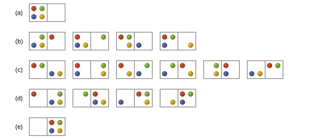
For this system, the most probable configuration is distribution (c) where the particles are evenly distributed between the boxes, that is, a configuration of two particles in each box. The probability of finding the system in this configuration is or [latex]\frac{6}{16}[/latex] or [latex]\frac{3}{8}[/latex]. The least probable configuration of the system is one in which all four particles are in one box, corresponding to distributions (a) and (e), each with a probability of [latex]\frac{1}{16}[/latex]. The probability of finding all particles in only one box (either the left box or right box) is then [latex](\frac{1}{16}\;+\;\frac{1}{16}) = \frac{2}{16}[/latex] or [latex]\frac{1}{8}[/latex].
As you add more particles to the system, the number of possible microstates increases exponentially (2N). A macroscopic (laboratory-sized) system would typically consist of moles of particles (N = ~ 1023), and the corresponding number of microstates would be staggeringly huge. Regardless of the number of particles in the system, however, the distributions in which roughly equal numbers of particles are found in each box are always the most probable configurations.
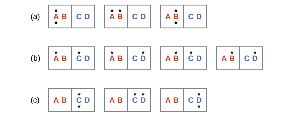
Consider a system consisting of two objects, each containing two particles, and two units of energy (represented as “*”) in Figure 3. The hot object is comprised of particles A and B and initially contains both energy units. The cold object is comprised of particles C and D, which initially has no energy units. Distribution (a) shows the three microstates possible for the initial state of the system, with both units of energy contained within the hot object. If one of the two energy units is transferred, the result is distribution (b) consisting of four microstates. If both energy units are transferred, the result is distribution (c) consisting of three microstates. And so, we may describe this system by a total of ten microstates. The probability that the heat does not flow when the two objects are brought into contact, that is, that the system remains in distribution (a), is [latex]\frac{3}{10}[/latex]. More likely is the flow of heat to yield one of the other two distribution, the combined probability being [latex]\frac{7}{10}[/latex]. The most likely result is the flow of heat to yield the uniform dispersal of energy represented by distribution (b), the probability of this configuration being [latex]\frac{4}{10}[/latex]. Extrapolating this treatment to macroscopic collections of particles dramatically increases the probability of the uniform distribution relative to the other distributions. This supports the common observation that placing hot and cold objects in contact results in spontaneous heat flow that ultimately equalizes the objects’ temperatures. And this spontaneous process is also characterized by an increase in system entropy.
Example 1
Determination of ΔS
Consider the system shown here. What is the change in entropy for a process that converts the system from distribution (left) to (right)?

Solution
We are interested in the following change:
The initial number of microstates is one, the final six:
The sign of this result is consistent with expectation; since there are more microstates possible for the final state than for the initial state, the change in entropy should be positive.
Check Your Learning
Consider the system shown in Figure 3. What is the change in entropy for the process where all the energy is transferred from the hot object (AB) to the cold object (CD)?
Answer:
0 J/K
Ch12.3 Predicting the Sign of ΔS
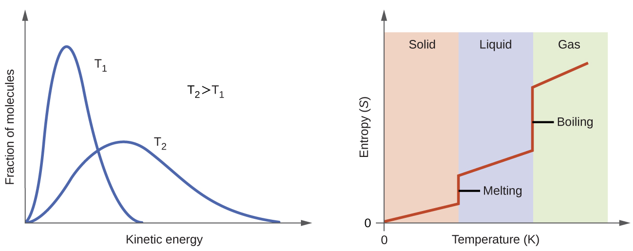
The relationships between entropy, microstates, and matter/energy dispersal described previously allow us to make generalizations regarding the relative entropies of substances and to predict the sign of entropy changes for chemical and physical processes. Consider the phase changes illustrated in Figure 4. In the solid phase, the molecules are restricted to nearly fixed positions with respect to each other and are capable of only modest oscillations about these positions. With essentially fixed locations for the system’s component particles, the number of microstates is relatively small. In the liquid phase, the molecules are free to move over and around each other, though they remain in relatively close proximity to one another. This increased freedom of motion results in a greater variation in possible particle locations, so the number of microstates is correspondingly greater than for the solid. As a result, Sliquid > Ssolid and the process of converting a substance from solid to liquid (melting) is characterized by an increase in entropy, ΔS > 0. By the same logic, the reciprocal process (freezing) exhibits a decrease in entropy, ΔS < 0.
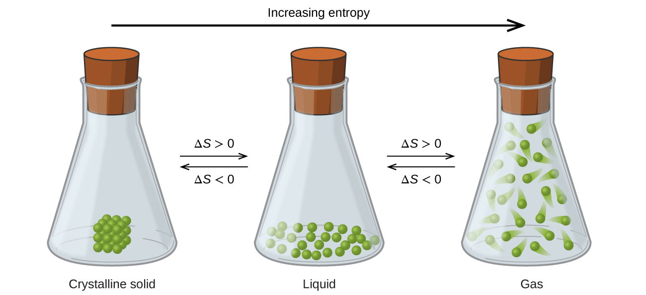
Now consider the vapor or gas phase. The molecules occupy a much greater volume than in the liquid phase; therefore each molecule can be found in many more locations than in the liquid (or solid) phase. Consequently, for any substance, Sgas > Sliquid > Ssolid, and the processes of vaporization and sublimation likewise involve increases in entropy, ΔS > 0. Likewise, the reciprocal phase transitions, condensation and deposition, involve decreases in entropy, ΔS < 0.
According to kinetic-molecular theory, the temperature of a substance is proportional to the average kinetic energy of its particles. At higher temperatures, the distribution of kinetic energies among the molecules of the substance is also broader (more dispersed) than at lower temperatures. Thus, the entropy for any substance increases with temperature (Figure 5).
The entropy of a substance is influenced by structure of the particles that comprise the substance. With regard to atomic substances, heavier atoms possess greater entropy at a given temperature than lighter atoms, which is a consequence of the relation between a particle’s mass and the spacing of quantized translational energy levels. For molecules, greater numbers of atoms (regardless of their masses) within the molecule increase the ways in which the molecules can vibrate and thus increase the number of possible microstates and the system’s entropy.
Finally, variations in the types of particles affects the entropy of a system. Compared to a pure substance, in which all particles are identical, the entropy of a mixture of two or more different particle types is greater. This is because of the additional orientations and interactions that are possible in a system comprised of nonidentical components. For example, when a solid dissolves in a liquid, the particles of the solid experience both a greater freedom of motion and additional interactions with the solvent particles. This corresponds to a more uniform dispersal of matter and energy and a greater number of microstates. The process of dissolution therefore involves an increase in entropy, ΔS > 0.
Considering the various factors that affect entropy allows us to make informed predictions of the sign of ΔS for various chemical and physical processes.
Example 2
Predicting the Sign of ∆S
Predict the sign of the entropy change for the following processes. Indicate the reason for each of your predictions.
(a) One mole liquid water at room temperature ⟶ one mole liquid water at 50 °C
(b) [latex]\text{Ag}^{+}(aq)\;+\;\text{Cl}^{-}(aq)\;{\longrightarrow}\;\text{AgCl}(s)[/latex]
(c) [latex]\text{C}_6\text{H}_6(l)\;+\;\frac{15}{2}\text{O}_2(g)\;{\longrightarrow}\;6\text{CO}_2(g)\;+\;3\text{H}_2\text{O}(l)[/latex]
(d) [latex]\text{NH}_3(s)\;{\longrightarrow}\;\text{NH}_3(l)[/latex]
Solution
(a) positive, temperature increases
(b) negative, reduction in the number of ions (particles) in solution, decreased dispersal of matter
(c) negative, net decrease in the amount of gaseous species
(d) positive, phase transition from solid to liquid, net increase in dispersal of matter
Check Your Learning
Predict the sign of the enthalpy change for the following processes. Give a reason for your prediction.
(a) [latex]\text{NaNO}_3(s)\;{\longrightarrow}\;\text{Na}^{+}(aq)\;+\;\text{NO}_3^{\;\;-}(aq)[/latex]
(b) the freezing of liquid water
(c) [latex]\text{CO}_2(s)\;{\longrightarrow}\;\text{CO}_2(g)[/latex]
(d) [latex]\text{CaCO}(s)\;{\longrightarrow}\;\text{CaO}(s)\;+\;\text{CO}_2(g)[/latex]
Answer:
(a) Positive; The solid dissolves to give an increase of mobile ions in solution. (b) Negative; The liquid becomes a more ordered solid. (c) Positive; The relatively ordered solid becomes a gas. (d) Positive; There is a net production of one mole of gas.
Ch12.4 Second Law of Thermodynamics
In the quest to identify a property that may reliably predict the spontaneity of a process, we have identified a very promising candidate: entropy. Processes that involve an increase in entropy of the system (ΔS > 0) are very often spontaneous; however, examples to the contrary are plentiful. By expanding consideration of entropy changes to include the surroundings, we may reach a significant conclusion regarding the relation between this property and spontaneity. In thermodynamic models, the system and surroundings comprise everything, that is, the universe, and so the following is true:
To illustrate this relation, consider again the process of heat flow between two objects, one identified as the system and the other as the surroundings. There are three possibilities for such a process:
- The objects are at different temperatures, and heat flows from the hotter to the cooler object. This is always observed to occur spontaneously. Designating the hotter object as the system and invoking the definition of entropy yields the following:
[latex]{\Delta}S_{\text{sys}} = \frac{-q_{\text{rev}}}{T_{\text{sys}}}\;\;\;\;\;\;\;\text{and}\;\;\;\;\;\;\;{\Delta}S_{\text{surr}} = \frac{q_{\text{rev}}}{T_{\text{surr}}}[/latex]
The arithmetic signs of qrev denote the loss of heat by the system and the gain of heat by the surroundings. Since Tsys > Tsurr in this scenario, the magnitude of the entropy change for the surroundings will be greater than that for the system, and so the sum of ΔSsys and ΔSsurr will yield a positive value for ΔSuniv. This process involves an increase in the entropy of the universe.
- The objects are at different temperatures, and heat flows from the cooler to the hotter object. This is never observed to occur spontaneously. Again designating the hotter object as the system and invoking the definition of entropy yields the following:
[latex]{\Delta}S_{\text{sys}} = \frac{q_{\text{rev}}}{T_{\text{sys}}}\;\;\;\;\;\;\;\text{and}\;\;\;\;\;\;\;{\Delta}S_{\text{surr}} = \frac{-q_{\text{rev}}}{T_{\text{surr}}}[/latex]
The arithmetic signs of qrev denote the gain of heat by the system and the loss of heat by the surroundings. The magnitude of the entropy change for the surroundings will again be greater than that for the system, but in this case, the signs of the heat changes will yield a negative value for ΔSuniv. This process involves a decrease in the entropy of the universe.
- The temperature difference between the objects is infinitesimally small, Tsys ≈ Tsurr, and so the heat flow is thermodynamically reversible. In this case, the system and surroundings experience entropy changes that are equal in magnitude and therefore sum to yield a value of zero for ΔSuniv. This process involves no change in the entropy of the universe.
These results lead to a profound statement regarding the relation between entropy and spontaneity known as the second law of thermodynamics: all spontaneous changes cause an increase in the entropy of the universe. A summary of these three relations is provided in Table 1.
| ΔSuniv > 0 | spontaneous |
| ΔSuniv < 0 | nonspontaneous (spontaneous in opposite direction) |
| ΔSuniv = 0 | reversible (system is at equilibrium) |
| Table 1. The Second Law of Thermodynamics | |
For many realistic applications, the surroundings are vast in comparison to the system. In such cases, the heat gained or lost by the surroundings as a result of some process represents a very small, nearly infinitesimal, fraction of its total thermal energy. For example, combustion of a fuel in air involves transfer of heat from a system (the fuel and oxygen molecules undergoing reaction) to surroundings that are infinitely more massive (the earth’s atmosphere). As a result, qsurr is a good approximation of qrev, and the second law may be stated as the following:
We may use this equation to predict the spontaneity of a process.
Example 3
Will Ice Spontaneously Melt?
The entropy change for the process
is 22.1 J/K and requires that the surroundings transfer 6.00 kJ of heat to the system. Is the process spontaneous at −10.00 °C? Is it spontaneous at +10.00 °C?
Solution
We can assess the spontaneity of the process by calculating the entropy change of the universe. If ΔSuniv is positive, then the process is spontaneous. At both temperatures, ΔSsys = 22.1 J/K and qsurr = −6.00 kJ.
At −10.00 °C (263.15 K):
ΔSuniv < 0, so melting is nonspontaneous at −10.0 °C.
At 10.00 °C (283.15 K):
ΔSuniv > 0, so melting is spontaneous at 10.00 °C.
Check Your Learning
Using this information, determine if liquid water will spontaneously freeze at the same temperatures. What can you say about the values of ΔSuniv?
Answer:
At −10.00 °C spontaneous, ΔSuniv = +0.7 J/K; at +10.00 °C nonspontaneous, ΔSuniv = −0.9 J/K. (Entropy is a state function, and freezing is the opposite of melting. )
Additionally, the entropy change for the surrounding can also be calculated from:
Hence, the ΔSuniverse can be expressed as:
The convenience of the above equation is that for a given reaction, ΔHsys = ΔHreaction, which can be calculated from the enthalphy of formation, ΔHf.
Ch12.5 Third Law of Thermodynamics
Consider the entropy of a pure, perfectly crystalline solid possessing no kinetic energy (that is, at a temperature of absolute zero, 0 K). This system may be described by a single microstate, as its purity, perfect crystallinity and complete lack of motion means there is but one possible location for each identical molecule comprising the crystal (W = 1). According to the Boltzmann equation, the entropy of this system is zero.
This limiting condition for a system’s entropy represents the third law of thermodynamics: the entropy of a pure, perfect crystalline substance at 0 K is zero.
We can make careful calorimetric measurements to determine the temperature dependence of a substance’s entropy and to derive absolute entropy values under specific conditions. Standard entropies are given the label [latex]S_{298}^{\circ}[/latex] for values determined for one mole of substance at a pressure of 1 bar and a temperature of 298 K. The standard entropy change (ΔS°) for any process may be computed from the standard entropies of its reactant and product species:
Here, ν represents stoichiometric coefficients in the balanced equation representing the process. For example, ΔS° for the following reaction at room temperature
is computed as the following:
The thermodynamics table in the appendix lists some standard entropies at 298.15 K.
Example 4
Determination of ΔS°
Calculate the standard entropy change for the following process:
Solution
The value of the standard entropy change at room temperature, [latex]{\Delta}S_{298}^{\circ}[/latex], is the difference between the standard entropy of the product, H2O(l), and the standard entropy of the reactant, H2O(g).
The value for [latex]{\Delta}S_{298}^{\circ}[/latex] is negative, as expected for this phase transition (condensation).
Check Your Learning
Calculate the standard entropy change for the following process:
Answer:
−120.6 J mol−1 K−1
Example 5
Determination of ΔS°
Calculate the standard entropy change for the combustion of methanol, CH3OH:
Solution
The value of the standard entropy change is equal to the difference between the standard entropies of the products and the entropies of the reactants scaled by their stoichiometric coefficients.
Check Your Learning
Calculate the standard entropy change for the following reaction:
Answer:
26.3 J/mol·K
Ch12.6 Gibbs Free Energy
One of the challenges of using the second law of thermodynamics to determine if a process is spontaneous is that we must determine the entropy change for the system and the entropy change for the surroundings. An alternative approach involving a new thermodynamic property defined in terms of system properties only was introduced in the late nineteenth century by American mathematician Josiah Willard Gibbs. This new property is called the Gibbs free energy change (G) (or simply the free energy), and it is defined in terms of a system’s enthalpy and entropy as the following:
Free energy is a state function, and at constant temperature and pressure, the change in standard free energy (ΔG°) may be expressed as the following:
We can derive this relationship from the second law expression:
The first law requires that qsurr = −qsys, and at constant pressure qsys = ΔHsys, and so this expression may be rewritten as:
Multiplying both sides of this equation by −T, and rearranging yields:
Comparing this equation to the one for free energy change shows the following relation:
The free energy change is therefore a reliable indicator of the spontaneity of a process, being directly related to ΔSuniv. Table 1 summarizes the relation between the spontaneity of a process and the arithmetic signs of these indicators.
| ΔSuniv > 0 | ΔG < 0 | spontaneous |
| ΔSuniv < 0 | ΔG > 0 | nonspontaneous |
| ΔSuniv = 0 | ΔG = 0 | reversible (at equilibrium) |
| Table 1. Relation between Process Spontaneity and Signs of Thermodynamic Properties | ||
Ch12.7 Calculating Free Energy Change
Free energy is a state function, so its value depends only on the conditions of the initial and final states of the system. A convenient and common approach to calculate free energy changes for physical and chemical reactions is by using standard state thermodynamic data. One method involves the use of standard enthalpies and entropies to compute standard free energy changes according to the relation:
Example 6
Evaluation of ΔG° Change from ΔH° and ΔS°
Use standard enthalpy and entropy data from Appendix to calculate the standard free energy change for the vaporization of water at room temperature (298 K). What does the computed value for ΔG° say about the spontaneity of this process?
Solution
The process of interest is the following:
From Appendix, the data is:
| Substance | [latex]{\Delta}H_{\text{f}}^{\circ}(\text{kJ/mol})[/latex] | [latex]S_{298}^{\circ}(\text{J/K}{\cdot}\text{mol})[/latex] |
|---|---|---|
| H2O(l) | −285.83 | 69.9 |
| H2O(g) | −241.82 | 188.8 |
At 298 K:
and:
Converting ΔS into kJ/mol·K and combining:
At 298 K (25 °C) [latex]{\Delta}G_{298}^{\circ}\;{\textgreater}\;0[/latex], therefore boiling is not spontaneous.
Check Your Learning
Use standard enthalpy and entropy data from Appendix to calculate the standard free energy change for the reaction shown below at 298 K. What does the computed value for ΔG° say about the spontaneity of this process?
Answer:
[latex]{\Delta}G_{298}^{\circ} = 101.0\;\text{kJ/mol}[/latex]; the reaction is nonspontaneous at 25 °C.
It is also possible to use the standard free energy of formation ([latex]{\Delta}G_{\text{f}}^{\circ}[/latex]) for each of the reactants and products involved in the reaction to calculate free energy changes. [latex]{\Delta}G_{\text{f}}^{\circ}[/latex] is the free energy change that accompanies the formation of one mole of a substance from its elements in their standard states. Similar to the standard enthalpies of formation, [latex]{\Delta}G_{\text{f}}^{\circ}[/latex] is by definition zero for elemental substances under standard state conditions. Similar to enthalpy and entropy changes, for a reaction:
the standard free energy change at room temperature would be:
Example 7
Calculation of [latex]{\Delta}G_{298}^{\circ}[/latex]
Consider the decomposition of yellow mercury(II) oxide.
Calculate [latex]{\Delta}G_{298}^{\circ}[/latex] using (a) standard free energies of formation and (b) standard enthalpies of formation and standard entropies. Do the results indicate the reaction to be spontaneous or nonspontaneous under these conditions?
Solution
The required data are available in Appendix and are shown here.
| Compound | [latex]{\Delta}G_{\text{f}}^{\circ}(\text{kJ/mol})[/latex] | [latex]{\Delta}H_{\text{f}}^{\circ}(\text{kJ/mol})[/latex] | [latex]S_{298}^{\circ}(\text{J/K}{\cdot}\text{mol})[/latex] |
|---|---|---|---|
| HgO (s, yellow) | −58.54 | −90.83 | 70.29 |
| Hg(l) | 0 | 0 | 76.02 |
| O2(g) | 0 | 0 | 205.1 |
(a) Using free energies of formation:
(b) Using enthalpies and entropies of formation:
Both calculation approach yield the same numerical value (to three significant figures), and both predict that the process is nonspontaneous at room temperature.
Check Your Learning
Calculate ΔG° using (a) free energies of formation and (b) enthalpies of formation and entropies (Appendix). Do the results indicate the reaction to be spontaneous or nonspontaneous at 25 °C?
Answer:
141.1 kJ/mol, nonspontaneous
Ch12.8 Temperature Dependence
As we’ve seen previously, the spontaneity of a process may depend upon the temperature of the system. Phase transitions, for example, will proceed spontaneously in one direction or the other depending on the temperature of the substance. Likewise, chemical reactions can exhibit temperature dependent spontaneities. Considered:
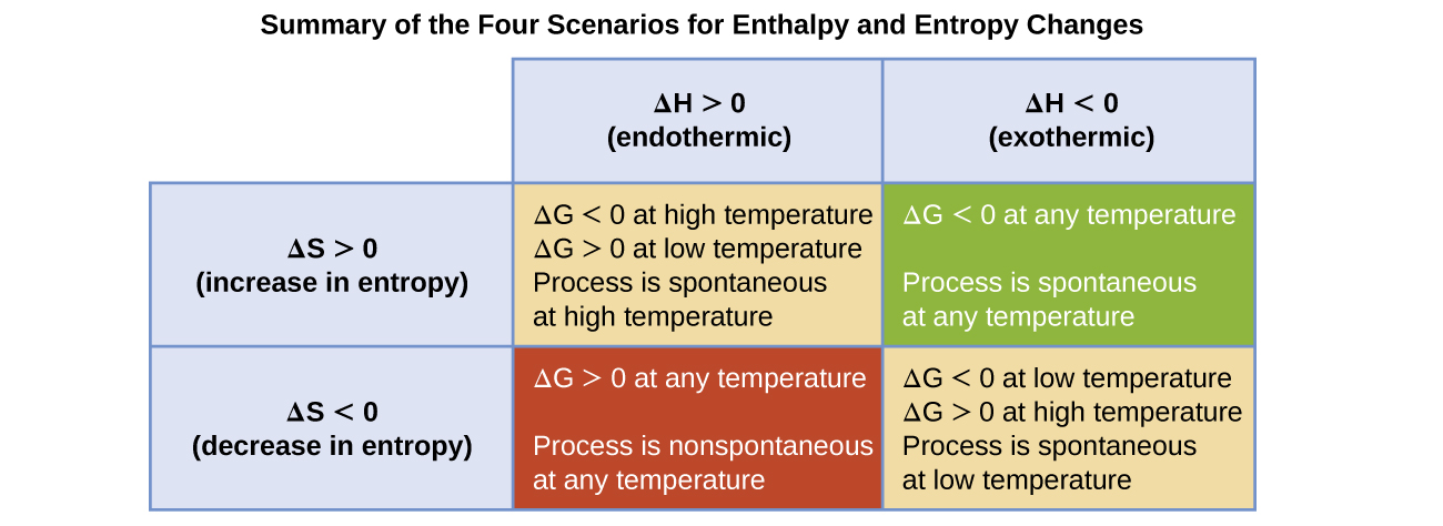
The spontaneity of a process, as reflected in the arithmetic sign of its free energy change, is determined by the signs of the enthalpy and entropy changes and, in some cases, the absolute (kelvin) temperature (T can only have positive values). Four possibilities therefore exist with regard to the signs of the enthalpy and entropy changes:
- Both ΔH and ΔS are positive. This condition describes an endothermic process that involves an increase in system entropy. In this case, ΔG will be negative if the magnitude of the TΔS term is greater than ΔH, and positive if the TΔS term is less than ΔH. Such a process is spontaneous at high temperatures and nonspontaneous at low temperatures.
- Both ΔH and ΔS are negative. This condition describes an exothermic process that involves a decrease in system entropy. In this case, ΔG will be negative if the magnitude of the TΔS term is less than ΔH and positive if the TΔS term is greater than ΔH. Such a process is spontaneous at low temperatures and nonspontaneous at high temperatures.
- ΔH is positive and ΔS is negative. This condition describes an endothermic process that involves a decrease in system entropy. In this case, ΔG will be positive regardless of the temperature. Such a process is nonspontaneous at all temperatures.
- ΔH is negative and ΔS is positive. This condition describes an exothermic process that involves an increase in system entropy. In this case, ΔG will be negative regardless of the temperature. Such a process is spontaneous at all temperatures.
These four scenarios are summarized in Figure 6.
Example 8
Predicting the Temperature Dependence of Spontaneity
The incomplete combustion of carbon is described by the following equation:
How does the spontaneity of this process depend upon temperature?
Solution
Combustion processes are exothermic (ΔH < 0). This particular reaction involves an increase in entropy due to the accompanying increase in the amount of gaseous species (net gain of one mole of gas, ΔS > 0). The reaction is therefore spontaneous (ΔG < 0) at all temperatures.
Check Your Learning
Popular chemical hand warmers generate heat by the air-oxidation of iron:
How does the spontaneity of this process depend upon temperature?
Answer:
ΔH and ΔS are negative; the reaction is spontaneous at low temperatures.
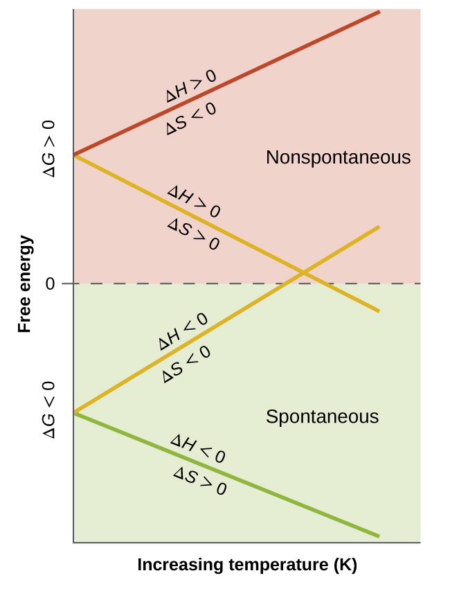
When considering the conclusions drawn regarding the temperature dependence of spontaneity, the temperatures in question are deemed “high” or “low” relative to some reference temperature. A process that is nonspontaneous at one temperature but spontaneous at another will necessarily undergo a change in “spontaneity” (as reflected by the sign of its ΔG) as temperature varies. This is illustrated by a graphical presentation of the free energy change equation, in which ΔG is plotted on the y axis versus T on the x axis (Figure 7):
A process whose enthalpy and entropy changes are of the same arithmetic sign will exhibit a temperature-dependent spontaneity as depicted by the two yellow lines in the plot. Each line crosses from one spontaneity domain (positive or negative ΔG) to the other at a temperature that is characteristic to the specific process. This temperature is represented by the x-intercept of the line, that is, the value of T for which ΔG is zero:
And so, saying a process is spontaneous at “high” or “low” temperatures means the temperature is above or below, respectively, that temperature at which ΔG for the process is zero.
Example 9
Equilibrium Temperature for a Phase Transition
The boiling point of a liquid is the temperature at which its solid and liquid phases are in equilibrium (when vaporization and condensation occur at equal rates) where ΔG = 0. Use the information in Appendix to estimate the boiling point of water.
Solution
The process of interest is the following phase change:
When ΔG° = 0:
Using the standard thermodynamic data from Appendix,
The accepted value for water’s normal boiling point is 373.2 K (100.0 °C), and so this calculation is in reasonable agreement. Note that the values for enthalpy and entropy changes data used were derived from standard data at 298 K (Appendix). If desired, you could obtain more accurate results by using enthalpy and entropy changes determined at (or at least closer to) the actual boiling point.
Check Your Learning
Use the information in Appendix to estimate the boiling point of CS2.
Answer:
320 K (accepted value 319 K)
