
Unit One
Day 3: Atomic Orbitals
As you work through this section, if you find that you need a bit more background material to help you understand the topics at hand, you can consult “Chemistry: The Molecular Science” (5th ed. Moore and Stanitski) Sections 5-4 through 5-6, and/or Chapter 2.1-2.7 in the Additional Reading Materials section.
D3.1 Atomic-Sized Particles Have Unusual Properties
Bohr’s model predicted experimental data for the hydrogen-atom emission spectra and was widely accepted, but it also raised questions. Why did electrons have energies defined by a single quantum number n = 1, 2, 3, and so on, but never in between? How could the model work so well for a hydrogen atom and one-electron ions, but not accurately predict the emission spectrum for helium or any atom or ion with two or more electrons? To answer such questions, we need to explore the unusual properties of matter at the atomic scale.
It is natural to try to interpret the behavior of electrons in atoms using analogies to the behavior of things we can see and experience. By the turn of the 20th century, scientists had identified two different kinds of behavior that might serve as analogies: waves and particles. Waves, such as water waves, can bend around objects and exhibit interference. A particle, such as a pea or tennis ball, moves in a straight line unless its path is changed by a force (such as friction, gravity, or hitting something). It turns out that properties of atomic-scale matter are best explained using a combination of these analogies.
Let’s think about an electron as if it were a particle and choose a very simple, but artificial, situation. Figure 1 shows an electron that is constrained to move in a single dimension, say the x direction. There are walls to the left and right of the electron that prevent it from moving beyond them; the distance between the walls is d (the electron is in a box of length d). Given an initial push, the electron will move back and forth forever (assuming no friction). The electron’s kinetic energy would be given by the equation $latexE = \frac{1}{2}m{v^2}$, where m is the mass and v the velocity.
Consider these questions regarding the electron moving in a one dimensional box:
But to explain the hydrogen-atom line spectrum, Bohr had to assume that an electron in an atom can only have certain energies. This assumption seemed very unsatisfactory based on the particle analogy—as we just saw, an electron should be able to have any energy value.
Let’s explore a wave analogy instead. In 1924, Louis de Broglie proposed that a wave of wavelength λ is associated with every particle. The larger the mass of the particle and the faster it is moving, the smaller this wavelength becomes. The relationship is given by the formula:
where μ is the momentum of the electron, the product of its mass and velocity ([latex]\mu = m\;\times\;v[/latex]), and h is Planck’s constant (h = 6.626 × 10⁻³⁴ J s).
Optional Information: Wavelike behavior of electrons was confirmed in 1927; read about it here. View this video for another description of the relevant experiments.
Suppose a wave, such as a vibrating guitar string, occupies the box. A guitar string is constrained by being fixed at each end so we assume the ends of the string are tied to the walls at the ends of the box.
In your course notebook, make a drawing of what a vibrating string of length d, with its ends in fixed positions, would look like. If you are studying with someone else, each make a drawing individually and then compare.
If an electron behaves like a guitar string, then only certain wavelengths will fit within the one-dimensional box with length d (see the figure in Activity 2). The length of the box can thus correspond to: a single half-wavelength, two half-wavelengths, three half-wavelengths, etc., but not to any wave where either end of the string is moving. In other words, the length d must correspond to an integer number of half wavelengths:
where n = 1, 2, 3, 4,… Solving the equation for [latex]\lambda[/latex], we obtain:
Combining this with de Broglie’s equation, [latex]\lambda = \dfrac{h}{\mu}[/latex], we have:
which rearranges to give:
We can now calculate the kinetic energy of our wave-particle. It is given by the formula:
Because n is a positive whole number, this equation says that the kinetic energy of the electron can have only certain values and not others.
Suppose an electron (m = 9.1 × 10⁻³¹ kg) is confined within a one-dimensional box about the size of an atom (d = 1.0 × 10⁻¹⁰ m). Calculate the lowest three allowed values of the energy. (Note that 1 J = 1 kg m2/s2; 1 aJ = 1 × 10-18 J )
This result shows that if we think of an electron as a wave in a 100 pm box, its energy is automatically restricted to certain specific values: the electron can have an energy of 6.0 attojoules (aJ) or 24.0 aJ, but not an intermediate energy such as 7.3 aJ or 11.6 aJ. We describe this situation by saying that the energy of the electron is quantized. Because the energy of 6.0 aJ is the lowest possible energy, the electron is most stable at this energy, where the box contains half a wavelength. This is the ground state. If the energy has a higher value, such as 24 aJ or 54 aJ, the electron is in an excited state. Notice that for the excited states the electron waves have one or more nodes. A node is a point where the wave has zero amplitude; that is, where the wave is not moving up or down at all. The greater the number of nodes, the higher the energy, a generalization that is true for all kinds of waves.
This new way of approaching the behavior of electrons (and other atomic-sized particles) became known as wave mechanics or quantum mechanics. Using both wave and particle analogies to describe atomic-scale matter is referred to as wave-particle duality. Wave-particle duality implies that we can no longer state that the electron is located at a specific position within the box or is moving in one direction or the other: the electron seems to be all over the box at once!
D3.2 The Heisenberg Uncertainty Principle
This inability to locate an electron precisely seems strange, but it is true of all atomic-scale particles. In 1927, Werner Heisenberg introduced the Heisenberg uncertainty principle: it is fundamentally impossible to determine simultaneously and exactly both the momentum and the position of a particle. Mathematically,
where Δx is the uncertainty in the position and Δpx is the uncertainty in the momentum along the x direction. Hence, the more accurately we measure the momentum of a particle, the less accurately we can determine its position at that time, and vice versa.
Exercise 3: Uncertainty Principle
Suppose we want to measure an electron’s position so that Δx = 1 pm (10–12 m, ~1% of the diameter of a hydrogen atom). Calculate the uncertainty in the electron’s momentum and velocity.
Δpx ≥ [number] × 10[exponent] kg m/s
Δvx ≥ [number] × 10[exponent] m/s
The result of your calculation shows that if an electron has Δx = 1 pm, the uncertainty in its velocity is at least 5 × 10⁷ m/s. In other words, we essentially have no idea how fast it’s moving.
Heisenberg’s principle imposes ultimate limits on what is measurable in science. It is possible to talk about the probability that the electron is at a specific location, or the probability that it is moving at a given speed, but there will also be some probability of finding it somewhere else in the box or moving at some other speed.
The uncertainty principle may seem strange, but we can say that the probability of finding a particle-like electron at a given location depends on the shape of the wave associated with the electron. The various wave shapes you drew in Activity 2 can be described mathematically using functions such as sines or cosines; that is, there is a mathematical wave function that describes each wave. The wave function is usually represented by a Greek letter $latex\psi$. Shortly after the uncertainty principle was proposed, the German physicist Max Born (1882 to 1969) suggested that the square of the magnitude of the wave function, [latex]|\psi|^2[/latex], at any position is proportional to the probability of finding the electron (as a particle) at that same position. If we can determine the wave function associated with an electron, we can also determine the relative probability of the electron’s being located at one point as opposed to another. Thus, each wave form you drew in Activity 2 can be represented by a different function, $latex\psi_n$, each has a different distribution of electric charge throughout the box, and each is associated with a different, specific energy value.
A graphic way of indicating the probability of finding the electron at a particular location is by the density of shading or stippling; that is, where the probability is high we draw lots of dots or darker shading and where the probability is low we draw fewer dots. We say that where the probability is high we have a large electron probability density (or just electron density). (In the guitar-string analogy we would draw lots of dots at places where the string was vibrating quite far from its rest position. For example, consider the wave shown below in red along with its square shown in blue. Wherever there is a maximum in the square of the wave function, we would plot a lot of dots.)
In your course notebook, annotate each of your drawings of the vibrating string with dots such that the density of dots indicates the electron probability density.
In Bohr’s theory an electron had a well-defined orbit around the nucleus, but according to the uncertainty principle, the best we can do is indicate electron density in various regions. Consequently we use a slightly different word to refer to the wave function and its electron-density distribution: orbital. The electron density of orbitals of an atom or molecule is very useful because it indicates where there is negative charge (electron density) relative to positive charge (atomic nuclei). This helps us understand atomic properties, chemical bonds, and forces between molecules.
D3.3 The Quantum–Mechanical Model of a Hydrogen Atom
If you think that an electron in a one-dimensional box is not a good model for an electron in an atom, that’s great, because the atom differs in two important ways: (1) the atom is three dimensional, so we have to consider motion of the electron, or electron waves, in three-dimensional space; and (2) the electron is not constrained by the ends of the box, which it cannot pass through, but rather is constrained by the force of electrostatic attraction between the electron’s negative charge and the positive charge of the nucleus (a proton in a hydrogen atom).
The force of attraction between a positive and a negative point electric charge (or the force of repulsion between two positive or two negative point charges) is given by Coulomb’s law:
In this equation ke is a proportionality constant equal to 8.99 × 10⁹ N m2 C−2, Q1 and Q2 are electric charge values, and r is the distance between the charges. For our purposes the energy of the pair of electric charges is more important than the force between them, so a second equation, which is derived from Coulomb’s law, is more useful:
Thus, the energy of two charged particles is proportional to the size of each charge and is inversely proportional to the distance between the charges. (Note that the energy equation differs from the force equation only in having r to the first power, instead of squared, in the denominator.) We often use this second equation qualitatively to predict the relative energies of electrons in atoms or the relative energies of ions in ionic compounds.
Exercise 4: Electrostatic Energy
For each of these pairs, identify the system with lower energy.
The fact that an atom is three-dimensional was addressed by Erwin Schrödinger, who viewed the electron in terms of three-dimensional stationary waves constrained by electrostatic attraction between electron and nucleus. When these wave functions were used to calculate allowed energies of a hydrogen atom, they reproduced Bohr’s expression for the energy levels:
Thus the wave theory correctly predicts the hydrogen-atom spectrum. The wave functions also define electron-density distributions. For a hydrogen atom in its ground state, the electron probability density distribution is shown in this video, where the hydrogen atom is rotated around its nucleus.
In your class notebook write a description of (1) the shape of the electron density distribution for a ground-state H atom and (2) how electron density changes with distance from the nucleus. (The nucleus is located at the intersection of the three axes: x, y, and z axes). In the electron-density diagram below, click on the white cross that corresponds to the lowest electron density.
Dot-density diagrams such as those in the video and Activity 4 are difficult to draw, so chemists usually use a different means of showing electron density distributions. A 3-D boundary-surface plot shows a surface that has the same shape as the electron density distribution and encloses some fraction, such as 90%, of the electron density. That is, if we could repeatedly locate the electron exactly, nine times out of ten the electron would be inside the boundary surface. This figure shows how a boundary surface is related to the dot-density plot you have already viewed. Move the slider at the bottom to change from dot-density to boundary-surface diagram.
Quantum Numbers: n, ℓ, mℓ
The wave functions of the three-dimensional standing waves of a hydrogen atom (the hydrogen-atom orbitals) can be defined using three quantum numbers: n, ℓ, and mℓ. Each wave function corresponds to an atomic orbital. Each atomic orbital defines a region in the atom within which electron probability density is large.
The energy of a hydrogen atom depends on the principal quantum number, n:
As n increases the size of the electron-density distribution also increases. Because the electron density is farther from the nucleus (corresponding to a larger r value in Exercise 4), the energy is higher (less negative): values of n>1 represent excited states of the atom. It is useful to think of the atom as consisting of shells of electron density: concentric spheres each farther from the nucleus. The orbitals that belong to a given shell have the same n and their electron density is the same distance from the nucleus. These boundary-surface diagrams show the relative sizes of the first three shells for a hydrogen atom:
The second quantum number, ℓ, the orbital quantum number (sometimes called azimuth or angular-momentum quantum number), determines the shape of the electron-density distribution. ℓ is an integer with values from zero up to n – 1; that is, ℓ= 0, 1, 2, …, n – 1. Thus, an orbital with n = 1 can have only one value of ℓ, ℓ = 0, whereas n = 2 permits ℓ = 0 and ℓ = 1, and so on. All orbitals with the same value of n and ℓ form a subshell.
Values of ℓ are designated using letters: orbitals with ℓ = 0 are called s orbitals; orbitals with ℓ = 1 are p orbitals; orbitals with ℓ = 2 are d orbitals, followed by the f, g, and h orbitals for ℓ = 3, 4, and 5. Each shell contains n subshells: for example, when n = 3, there is a 3s subshell, a 3p subshell, and a 3d subshell, corresponding to the three possible ℓ values of 0, 1 and 2.
View the shapes of s, p, and d orbitals shown in these videos: 1s orbital 2p orbital 3d orbital
In your class notebook write a description of the shape of the electron density distribution for each orbital. Also, make a rough drawing of the corresponding boundary-surface diagram for each dot-density diagram.
The colors of dots in these dot-density diagrams represent the mathematical sign of the wave function. Where the color changes from blue to red the wave function changes from a positive value to a negative value; that is, the wave function value passes through zero, indicating a node in the wave function. For the particle in a box, more nodes corresponded to higher energy. Is that true for the hydrogen atom also? Write an explanation in your class notebook.
The magnetic quantum number, mℓ, specifies the spatial orientation of a particular orbital. Values of mℓ can be any integer from –ℓ, up to ℓ. For example, for an s orbital, ℓ = 0, and the only value of mℓ is zero; thus an s subshell contains a single orbital. For p orbitals, ℓ = 1, and mℓ can be equal to –1, 0, or +1; thus a p subshell can contain three different p orbitals, px, py, and pz, which are oriented along the x, y, and z axes. The total number of possible orbitals with the same value of ℓ (the number of orbitals in a subshell) is 2ℓ + 1. There are five d orbitals, seven f orbitals, and so forth. The sizes and shapes of s, p, and d orbitals in the first three shells are shown in Figure 2. Each of these orbitals corresponds to a different set of the three values of n, ℓ, and mℓ.
Spin Quantum Number, ms
When hydrogen-atom line spectra are examined at extremely high resolution, pairs of closely spaced lines are observed. This so-called fine structure implies that even when an electron is in the same orbital (when the same values of n, ℓ, and mℓ are assigned) there can be a small difference in energy. These observations led Samuel Goudsmit and George Uhlenbeck to propose a fourth quantum number: the spin quantum number, ms. Each electron acts as if it were a tiny rotating charged object with an angular momentum; that is, as if it were a tiny magnet. The magnitude of the overall electron spin can only have one value, and an electron can only spin in one of two quantized states characterized by two values of the quantum number: [latex]m_s = \frac{1}{2}[/latex] or [latex]m_s = -\frac{1}{2}[/latex].
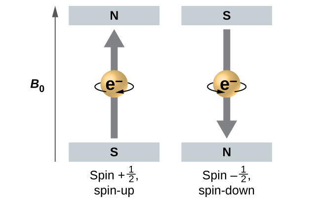
A magnet has a lower energy if its magnetic moment is aligned with the external magnetic field (the left electron on Figure 3) and a higher energy if its magnetic moment is opposite to the applied field. For orbitals other than s orbitals in a hydrogen atom the electron’s orbital motion produces a magnetic field, so the electron’s internal magnetic moment can either align with or oppose that magnetic field. This gives a very slightly different electron energy for [latex]m_s = \frac{1}{2}[/latex] compared to [latex]m_s = -\frac{1}{2}[/latex]. Consequently there are two possible electron transitions to the ground state, each corresponding to a slightly different energy (and hence wavelength). The line in the spectrum shows a fine-structure splitting.
In your class notebook make a table summarizing the names, symbols, allowed values, and important properties of the four quantum numbers as applied to atoms with more than a single electron. (You can use this table for studying later.)
If you are studying with someone else, make your tables independently and then compare. When you are satisfied with your table, compare it with ours by clicking here.
At the beginning of this section you were asked to write down what you remembered about atomic orbitals and quantum numbers and note any aspects of atomic orbitals that puzzle you. Review what you wrote and rewrite it so that it provides a good summary you can use to review later as you study for an exam.
Podia Question
Consider these two sentences: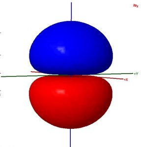
- The surface shown in this illustration of an atomic orbital is chosen so that the entirety of the electron’s wave function is enclosed.
- The colors in the diagram represent regions of opposite electron spin.
Decide whether each sentence is correct. Rewrite all incorrect text so that it is correct. Be brief but include all important ideas and use scientifically appropriate language.
Two days before the next whole-class session, this Podia question will become live on Podia, where you can submit your answer.
