
Additional Reading Materials
Chapter 9: Reaction Rates and Kinetics
Ch9.1 Reaction Rate
A rate is a measure of how some property varies with time. Speed is a rate that expresses the distance traveled by an object in a given amount of time. Wage is a rate that represents the amount of money earned by a person working for a given amount of time.
The rate of a reaction is the change in the amount of a reactant or a product per unit time. Reaction rates are therefore determined by measuring the time dependence of some property that can be related to the amount of reactant or product. For example, rates of reactions that consume or produce gaseous substances can be determined by measuring changes in volume or pressure. For reactions involving one or more colored substances, rates may be monitored via measurements of light absorption. For reactions involving aqueous electrolytes, rates may be measured via changes in a solution’s conductivity.
For reactants and products in solution, their relative amounts (concentrations) are used for purposes of expressing reaction rates. If we measure the concentration of hydrogen peroxide, H2O2, in an aqueous solution, we find that it changes slowly over time as the H2O2 decomposes, according to the equation:
2H2O2(aq) → 2H2O(l) + O2(g)
The rate at which the hydrogen peroxide decomposes can be expressed in terms of the rate of change of its concentration, as shown here:
This mathematical representation of the change in species concentration over time is the rate expression for the reaction. The brackets indicate molar concentrations, and the symbol delta (Δ) indicates “change in.” Thus, [H2O2]t1 represents the molar concentration of hydrogen peroxide at some time t1; [H2O2]t2 represents the molar concentration of hydrogen peroxide at a later time t2; and Δ[H2O2] represents the change in molar concentration of hydrogen peroxide during the time interval Δt (that is, t2 − t1). Since the reactant concentration decreases as the reaction proceeds, Δ[H2O2] is a negative quantity; we place a negative sign in front of the expression because reaction rates are, by convention, positive quantities. Figure 1 provides an example of data collected during the decomposition of H2O2.
![A table with five columns is shown. The first column is labeled, “Time, h.” Beneath it the numbers 0.00, 6.00, 12.00, 18.00, and 24.00 are listed. The second column is labeled, “[ H subscript 2 O subscript 2 ], mol / L.” Below, the numbers 1.000, 0.500, 0.250, 0.125, and 0.0625 are double spaced. To the right, a third column is labeled, “capital delta [ H subscript 2 O subscript 2 ], mol / L.” Below, the numbers negative 0.500, negative 0.250, negative 0.125, and negative 0.062 are listed such that they are double spaced and offset, beginning one line below the first number listed in the column labeled, “[ H subscript 2 O subscript 2 ], mol / L.” The first two numbers in the second column have line segments extending from their right side to the left side of the first number in the third row. The second and third numbers in the second column have line segments extending from their right side to the left side of the second number in the third row. The third and fourth numbers in the second column have line segments extending from their right side to the left side of the third number in the third row. The fourth and fifth numbers in the second column have line segments extending from their right side to the left side of the fourth number in the third row. The fourth column in labeled, “capital delta t, h.” Below the title, the value 6.00 is listed four times, each single-spaced. The fifth and final column is labeled “Rate of Decomposition, mol / L / h.” Below, the following values are listed single-spaced: negative 0.0833, negative 0.0417, negative 0.0208, and negative 0.0103.](https://wisc.pb.unizin.org/app/uploads/sites/126/2017/08/CNX_Chem_12_01_KDataH2O2.jpg)
The concentration of hydrogen peroxide was measured every 6 hours over the course of a day at a constant temperature of 40 °C. Reaction rates were computed for each time interval by dividing the change in concentration by the corresponding time increment, as shown here for the first 6-hour period:
Notice that the reaction rates vary with time, decreasing as the reaction proceeds. Results for the last 6-hour period yield a reaction rate of:
Using the concentrations at the beginning and end of a time period over which the reaction rate is changing results in the calculation of an average rate for the reaction over this time interval. At any specific time, the rate at which a reaction is proceeding is known as its instantaneous rate. The instantaneous rate of a reaction at “time zero,” when the reaction commences, is its initial rate. Consider the analogy of a car slowing down as it approaches a stop sign. The vehicle’s initial speed would be the speedometer reading at the moment the driver begins pressing the brakes (t0). A few moments later, the instantaneous speed at a specific moment (t1) would be somewhat slower, as indicated by the speedometer reading at that point in time. As time passes, the instantaneous speed will continue to fall until it reaches zero when the car stops. Unlike instantaneous speed, the car’s average speed is not indicated by the speedometer; but it can be calculated as the ratio of the distance traveled to the time required to bring the vehicle to a complete stop.
The instantaneous rate of a reaction may be determined one of two ways. If experimental conditions permit the measurement of concentration changes over very short time intervals, then average rates over these very short time intervals provide reasonably good approximations of instantaneous rates. Alternatively, a graphical procedure may be used. If we plot the concentration of hydrogen peroxide against time, the instantaneous rate of decomposition of H2O2 at any time t is given by the slope of a straight line that is tangent to the curve at that time (Figure 2). We can use calculus to evaluating the slopes of such tangent lines.
![A graph is shown with the label, “Time ( h ),” appearing on the x-axis and “[ H subscript 2 O subscript 2 ] ( mol L superscript negative 1)” on the y-axis. The x-axis markings begin at 0 and end at 24. The markings are labeled at intervals of 6. The y-axis begins at 0 and includes markings every 0.200, up to 1.000. A decreasing, concave up, non-linear curve is shown, which begins at 1.000 on the y-axis and nearly reaches a value of 0 at the far right of the graph around 10 on the x-axis. A red tangent line segment is drawn on the graph at the point where the graph intersects the y-axis. A second red tangent line segment is drawn near the middle of the curve. A vertical dashed line segment extends from the left endpoint of the line segment downward to intersect with a similar horizontal line segment drawn from the right endpoint of the line segment, forming a right triangle beneath the curve. The vertical leg of the triangle is labeled “capital delta [ H subscript 2 O subscript 2 ]” and the horizontal leg is labeled, “capital delta t.”](https://wisc.pb.unizin.org/app/uploads/sites/126/2017/08/CNX_Chem_12_01_RRateIll.jpg)
Reaction Rates in Analysis: Test Strips for Urinalysis
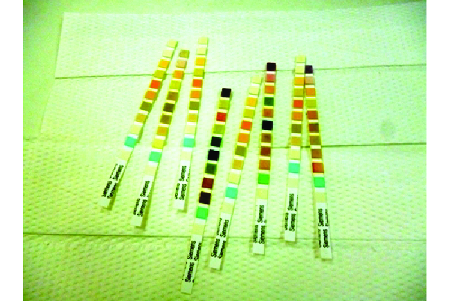
Physicians often use disposable test strips to measure the amounts of various substances in a patient’s urine (Figure 3). These test strips contain various chemical reagents, embedded in small pads at various locations along the strip, which undergo changes in color upon exposure to sufficient concentrations of specific substances. The usage instructions for test strips often stress that proper read time is critical for optimal results. This emphasis on read time suggests that kinetic aspects of the chemical reactions occurring on the test strip are important considerations.
The test for urinary glucose relies on a two-step process represented by the chemical equations shown here:
The first equation depicts the oxidation of glucose to form glucolactone and hydrogen peroxide. The hydrogen peroxide subsequently oxidizes colorless iodide ion to yield brown iodine, which may be visually detected. Some strips include an additional substance that reacts with iodine to produce a more distinct color change.
The two reactions above are inherently very slow, but their rates are increased by special enzymes embedded in the test strip pad. This is an example of catalysis, a topic that will be discussed later. A typical glucose test strip for use with urine requires approximately 30 seconds for completion of the color-forming reactions. Reading the result too soon might lead one to conclude that the glucose concentration of the urine sample is lower than it actually is (a false-negative result). Waiting too long to assess the color change can lead to a false positive due to the slower (not catalyzed) oxidation of iodide ion by other substances found in urine.
Ch9.2 Relative Rates of Reaction
The rate of a reaction may be expressed in terms of the change in the amount of any reactant or product, and may be simply derived from the stoichiometry of the reaction. Consider the reaction represented by the following equation:
2NH3(g) → N2(g) + 3H2(g)
The stoichiometric factors derived from this equation may be used to relate reaction rates in the same manner that they are used to related reactant and product amounts. The relation between the reaction rates expressed in terms of nitrogen production and ammonia consumption, for example, is:
Or:
Note that the negative sign accounts for the opposite signs of the two amount changes (the reactant amount is decreasing while the product amount is increasing).
If the reactants and products are present in the same solution, the molar amounts may be replaced by concentrations:
Similarly, the rate of formation of H2 is three times the rate of formation of N2 because three moles of H2 form during the time required for the formation of one mole of N2:
Figure 4 illustrates the change in concentrations over time for the decomposition of ammonia into nitrogen and hydrogen at 1100 °C. We can see from the slopes of the tangents drawn at t = 500 seconds that the instantaneous rates of change in the concentrations of the reactants and products are related by their stoichiometric factors. The rate of hydrogen production, for example, is observed to be three times greater than that for nitrogen production:
![A graph is shown with the label, “Time ( s ),” appearing on the x-axis and, “Concentration ( M ),” on the y-axis. The x-axis markings begin at 0 and end at 2000. The markings are labeled at intervals of 500. The y-axis begins at 0 and includes markings every 1.0 times 10 superscript negative 3, up to 4.0 times 10 superscript negative 3. A decreasing, concave up, non-linear curve is shown, which begins at about 2.8 times 10 superscript negative 3 on the y-axis and nearly reaches a value of 0 at the far right of the graph at the 2000 marking on the x-axis. This curve is labeled, “[ N H subscript 3].” Two additional curves that are increasing and concave down are shown, both beginning at the origin. The lower of these two curves is labeled, “[ N subscript 2 ].” It reaches a value of approximately 1.25 times 10 superscript negative 3 at 2000 seconds. The final curve is labeled, “[ H subscript 2 ].” It reaches a value of about 3.9 times 10 superscript negative 3 at 2000 seconds. A red tangent line segment is drawn to each of the curves on the graph at 500 seconds. At 500 seconds on the x-axis, a vertical dashed line is shown. Next to the [ N H subscript 3] graph appears the equation “negative capital delta [ N H subscript 3 ] over capital delta t = negative slope = 1.94 times 10 superscript negative 6 M / s.” Next to the [ N subscript 2] graph appears the equation “negative capital delta [ N subscript 2 ] over capital delta t = negative slope = 9.70 times 10 superscript negative 7 M / s.” Next to the [ H subscript 2 ] graph appears the equation “negative capital delta [ H subscript 2 ] over capital delta t = negative slope = 2.91 times 10 superscript negative 6 M / s.”](https://wisc.pb.unizin.org/app/uploads/sites/126/2017/08/CNX_Chem_12_01_NH3Decomp.jpg)
Example 1
Expressions for Relative Reaction Rates
The first step in the production of nitric acid is the combustion of ammonia:
4NH3(g) + 5O2(g) → 4NO(g) + 6H2O(g)
Write the equations that relate the rates of consumption of the reactants and the rates of formation of the products.
Solution
Considering the stoichiometry of this homogeneous reaction, the rates for the consumption of reactants and formation of products are:
Check Your Learning
In a reaction described by the following net ionic equation:
5Br– + BrO3– + 6H+ → 3Br2 + 3H2O
Write the equations that relate the rates of consumption of the reactants and the rates of formation of the products.
Answer:
[latex]-\frac{1}{5}\;\frac{{\Delta}[\text{Br}^{-}]}{{\Delta}t} = -\frac{{\Delta}[\text{BrO}_3^{\;\;-}]}{{\Delta}t} = -\frac{1}{6}\;\frac{{\Delta}[\text{H}^{+}]}{{\Delta}t} = \frac{1}{3}\;\frac{{\Delta}[\text{Br}_2]}{{\Delta}t} = \frac{1}{3}\;\frac{{\Delta}[\text{H}_2\text{O}]}{{\Delta}t}[/latex]
Example 2
Reaction Rate Expressions for Decomposition of H2O2
The graph in Figure 2 shows the rate of the decomposition of H2O2 over time:
2H2O2(aq) → 2H2O(l) + O2(g)
Based on these data, the instantaneous rate of decomposition of H2O2 at t = 11.1 h is determined to be 3.20 × 10⁻² M/h. What is the instantaneous rate of production of H2O and O2 at t = 11.1 h?
Solution
Using the stoichiometry of the reaction, we may determine that:
Therefore:
and
Check Your Learning
If the rate of decomposition of ammonia, NH3, at 1150 K is 2.10 × 10⁻⁶ M/s, what is the rate of production of nitrogen and hydrogen?
Answer:
1.05 × 10⁻⁶ M/s for N2 and 3.15 × 10⁻⁶ M/s for H2.
Ch9.3 Factors Affecting Reaction Rates
The Chemical Nature of the Reacting Substances
The rate of a reaction depends on the nature of the participating substances. Reactions that appear similar may have different rates under the same conditions, depending on the identity of the reactants. For example, when small pieces of the metals iron and sodium are exposed to air, the sodium reacts completely with air overnight, whereas the iron is barely affected. The active metals calcium and sodium both react with water to form hydrogen gas and a base. Yet calcium reacts at a moderate rate, whereas sodium reacts so rapidly that the reaction is almost explosive.
The State of Subdivision of the Reactants
Except for substances in the gaseous state or in solution, reactions occur at the boundary, or interface, between two phases. Hence, the rate of a reaction between two phases depends to a great extent on the surface contact between them. A finely divided solid has more surface area available for reaction than does one large piece of the same substance. For example, large pieces of iron react slowly with acids; finely divided iron reacts much more rapidly (Figure 5). Large pieces of wood smolder, smaller pieces burn rapidly, and saw dust burns explosively.
Watch this video to see the reaction of cesium with water in slow motion and a discussion of how the state of reactants and particle size affect reaction rates.
Temperature of the Reaction
Chemical reactions typically occur faster at higher temperatures. Food can spoil quickly when left on the kitchen counter. However, the lower temperature inside of a refrigerator slows that process so that the same food remains fresh for days. We use a burner or a hot plate in the laboratory to increase the speed of reactions that proceed slowly at room temperature. In many cases, an increase in temperature of only 10 °C will approximately double the rate of a reaction in a homogeneous system.
Concentrations of the Reactants
Rates usually increase when the concentration of one or more of the reactants increases. For example, calcium carbonate (CaCO3) deteriorates as a result of its reaction with the pollutant sulfur dioxide. The rate of this reaction depends on the amount of acidic sulfur dioxide in the air (Figure 6), which reacts with water vapor to produce sulfurous acid:
SO2(g) + H2O(g) → H2SO3(aq)
Calcium carbonate then reacts with sulfurous acid:
CaCO3(s) + H2SO3(aq) → CaSO3(aq) + CO2(g) + H2O(l)
In a more polluted atmosphere where the concentration of sulfur dioxide is higher, calcium carbonate deteriorates more rapidly.

Similarly, phosphorus burns much more rapidly in an atmosphere of pure oxygen than in air, which is only about 20% oxygen.
Phosphorous burns rapidly in air, but it will burn even more rapidly if the concentration of oxygen in is higher. Watch this video to see an example.
Presence of a Catalyst
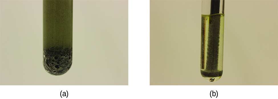
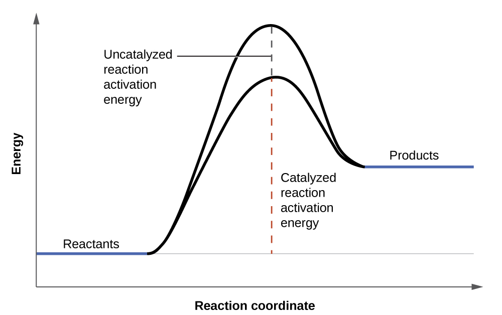
Hydrogen peroxide solutions foam when poured onto an open wound because substances in the exposed tissues act as catalysts, increasing the rate of hydrogen peroxide’s decomposition. However, in the absence of these catalysts (for example, in the bottle in the medicine cabinet) complete decomposition can take months. A catalyst is a substance that increases the rate of a chemical reaction by lowering the activation energy without itself being consumed by the reaction. Activation energy is the minimum amount of energy required for a chemical reaction to proceed in the forward direction. A catalyst increases the reaction rate by providing an alternative pathway or mechanism for the reaction to follow (Figure 7). Catalysis will be discussed in greater detail later.
Chemical reactions occur when molecules collide with each other and undergo a chemical transformation. Before physically performing a reaction in a laboratory, scientists can use molecular modeling simulations to predict how the parameters discussed earlier will influence the rate of a reaction. Use the PhET Reactions & Rates interactive to explore how temperature, concentration, and the nature of the reactants affect reaction rates.
Ch9.4 Rate Laws
Rate laws or rate equations are mathematical expressions that describe the relationship between the rate of a chemical reaction and the concentration of its reactants. In general, a rate law (or differential rate law, as it is sometimes called) takes this form:
rate = k[A]m[B]n[C]p…
in which [A], [B], and [C] represent the molar concentrations of reactants, and k is the rate constant, which is specific for a particular reaction at a particular temperature. The exponents m, n, and p are usually positive integers (although it is possible for them to be fractions or negative numbers). The rate constant k and the exponents m, n, and p must be determined experimentally by observing how the rate of a reaction changes as the concentrations of the reactants are changed. The rate constant k is independent of the concentration of A, B, or C, but it does vary with temperature and surface area.
The exponents in a rate law describe the effects of the reactant concentrations on the reaction rate and define the reaction order. Consider a reaction for which the rate law is:
rate = k[A]m[B]n
If the exponent m is 1, the reaction is first order with respect to A. If m is 2, the reaction is second order with respect to A. If n is 1, the reaction is first order in B. If n is 2, the reaction is second order in B. If m or n is zero, the reaction is zero order in A or B, respectively, and the rate of the reaction is not affected by the concentration of that reactant. The overall reaction order is the sum of the orders with respect to each reactant. If m = 1 and n = 1, the overall order of the reaction is second order (m + n = 1 + 1 = 2).
The rate law:
rate = k[H2O2]
describes a reaction that is first order in hydrogen peroxide and first order overall. The rate law:
rate = k[C4H6]2
describes a reaction that is second order in C4H6 and second order overall. The rate law:
rate = k[H+][OH–]
describes a reaction that is first order in H+, first order in OH−, and second order overall.
Example 3
Writing Rate Laws from Reaction Orders
An experiment shows that the reaction of nitrogen dioxide with carbon monoxide:
NO2(g) + CO(g) → NO(g) + CO2(g)
is second order in NO2 and zero order in CO at 100 °C. What is the rate law for the reaction?
Solution
The reaction will have the form:
rate = k[NO2]m[CO]n
The reaction is second order in NO2; thus m = 2. The reaction is zero order in CO; thus n = 0. The rate law is:
rate = k[NO2]2[CO]0 = k[NO2]2
Remember that a number raised to the zero power is equal to 1, thus [CO]0 = 1, which is why we can simply drop the concentration of CO from the rate equation: the rate of reaction is solely dependent on the concentration of NO2. When we consider rate mechanisms later on, we will explain how a reactant’s concentration can have no effect on a reaction despite being involved in the reaction.
Check Your Learning
The rate law for the reaction:
H2(g) + 2NO(g) → N2O(g) + H2O(g)
has been determined to be rate = k[NO]2[H2]. What are the orders with respect to each reactant, and what is the overall order of the reaction?
Answer:
order in NO = 2; order in H2 = 1; overall order = 3
Check Your Learning
In a transesterification reaction, a triglyceride reacts with an alcohol to form an ester and glycerol. Many students learn about the reaction between methanol (CH3OH) and ethyl acetate (CH3CH2OCOCH3) as a sample reaction before studying the chemical reactions that produce biodiesel:
CH3OH + CH3CH2OCOCH3 → CH3OCOCH3 + CH3CH2OH
The rate law for this reaction, under certain conditions, is determined to be:
rate = k[CH3OH]
What is the order of reaction with respect to methanol and ethyl acetate, and what is the overall order of reaction?
Answer:
order in CH3OH = 1; order in CH3CH2OCOCH3 = 0; overall order = 1
It is sometimes helpful to use a more explicit algebraic method, often referred to as the method of initial rates, to determine the orders in rate laws. To use this method, we select two sets of rate data that differ in the concentration of only one reactant and set up a ratio of the two rates and the two rate laws. After canceling terms that are equal, we are left with an equation that contains only one unknown, the coefficient of the concentration that varies. We then solve this equation for the coefficient.
Example 4
Determining a Rate Law from Initial Rates
Ozone in the upper atmosphere is depleted when it reacts with nitrogen oxides. The rates of the reactions of nitrogen oxides with ozone are important factors in deciding how significant these reactions are in the formation of the ozone hole over Antarctica (Figure 8).

One such reaction is the combination of nitric oxide, NO, with ozone, O3:
NO(g) + O3(g) → NO2(g) + O2(g)
This reaction has been studied in the laboratory, and the following rate data were determined at 25 °C.
| Trial | [NO] (M) | [O3] (M) | [latex]\frac{{\Delta}[\text{NO}_2]}{{\Delta}t}\;(\text{M/s})[/latex] |
|---|---|---|---|
| 1 | 1.00 × 10⁻⁶ | 3.00 × 10⁻⁶ | 6.60 × 10⁻⁵ |
| 2 | 1.00 × 10⁻⁶ | 6.00 × 10⁻⁶ | 1.32 × 10⁻⁴ |
| 3 | 1.00 × 10⁻⁶ | 9.00 × 10⁻⁶ | 1.98 × 10⁻⁴ |
| 4 | 2.00 × 10⁻⁶ | 9.00 × 10⁻⁶ | 3.96 × 10⁻⁴ |
| 5 | 3.00 × 10⁻⁶ | 9.00 × 10⁻⁶ | 5.94 × 10⁻⁴ |
Determine the rate law and the rate constant for the reaction at 25 °C.
Solution
The rate law will have the form:
rate = k[NO]m[O3]n
We can determine the values of m, n, and k from the experimental data using the following three-part process:
- Determine the value of m from the data in which [NO] varies and [O3] is constant.
- When [NO] doubles from trial 3 to 4, the rate doubles, and when [NO] triples from trial 3 to 5, the rate also triples. Thus, the rate is also directly proportional to [NO], and m = 1.
- Determine the value of n from data in which [O3] varies and [NO] is constant.
- The reaction rate changes in direct proportion to the change in [O3]. When [O3] doubles from trial 1 to 2, the rate doubles; when [O3] triples from trial 1 to 3, the rate increases also triples. Thus, the rate is directly proportional to [O3], and n = 1.
- The rate law is thus: rate = k[NO]1[O3]1
- Determine the value of k from one set of concentrations and the corresponding rate.
[latex]\begin{array}{r @{{}={}} l} k & \frac{\text{rate}}{[\text{NO}][\text{O}_3]} \\[0.5em] & \frac{6.60\;\times\;10^{-5}\;\rule[0.5ex]{0.7em}{0.1ex}\hspace{-0.7em}\text{M}\text{s}^{-1}}{(1.00\;\times\;10^{-6}\;\rule[0.5ex]{0.7em}{0.1ex}\hspace{-0.7em}\text{M})(3.00\;\times\;10^{-6}\;\text{M})} \\[0.5em] & 2.20\;\times\;10^{7}\;\text{M}^{-1}\text{s}^{-1} \end{array}[/latex]
The large value of k tells us that this is a fast reaction that could play an important role in ozone depletion if [NO] is large enough.
Check Your Learning
Acetaldehyde decomposes when heated to yield methane and carbon monoxide according to the equation:
CH3CHO(g) → CH4(g) + CO(g)
Determine the rate law and the rate constant for the reaction from the following experimental data:
| Trial | [CH3CHO] (M) | [latex]-\frac{{\Delta}[\text{CH}_3\text{CHO}]}{{\Delta}t}\;(\text{M/s})[/latex] |
|---|---|---|
| 1 | 1.75 × 10⁻³ | 2.06 × 10⁻¹¹ |
| 2 | 3.50 × 10⁻³ | 8.24 × 10⁻¹¹ |
| 3 | 7.00 × 10⁻³ | 3.30 × 10⁻¹⁰ |
Answer:
rate = k[CH3CHO]2, with k = 6.73 × 10⁻⁶ [latex]\frac{1}{M*s}[/latex]
Example 5
Determining Rate Laws from Initial Rates
Using the initial rates method and the experimental data, determine the rate law and the value of the rate constant for this reaction:
2NO(g) + Cl2(g) → 2NOCl(g)
| Trial | [NO] (M) | [Cl2] (M) | [latex]-\frac{{\Delta}[\text{NO}]}{{\Delta}t}\;(\text{M/s})[/latex] |
|---|---|---|---|
| 1 | 0.10 | 0.10 | 0.00300 |
| 2 | 0.10 | 0.15 | 0.00450 |
| 3 | 0.15 | 0.10 | 0.00675 |
Solution
The rate law for this reaction will have the form:
rate = k[NO]m[Cl2]n
We can again approach this problem in a stepwise fashion, determining the values of m and n from the experimental data and then using these values to determine the value of k. In this example, however, we will use a different approach to determine the values of m and n:
- Determine the value of m from the data in which [NO] varies and [Cl2] is constant.
- We can write the ratios with the subscripts x and y to indicate data from two different trials:
[latex]\frac{\text{rate}_x}{\text{rate}_y} = \frac{k[\text{NO}]_x^m[\text{Cl}_2]_x^n}{k[\text{NO}]_y^m[\text{Cl}_2]_y^n}[/latex]
Using trial 3 and 1, in which [Cl2] does not vary, gives:
[latex]\frac{\text{rate}\;3}{\text{rate}\;1} = \frac{0.00675\;\text{M/s}}{0.00300\;\text{M/s}} = \frac{k(0.15\;\text{M})^m(0.10\;\text{M})^n}{k(0.10\;\text{M})^m(0.10\;\text{M})^n}[/latex]After canceling equivalent terms in the numerator and denominator, we are left with:
[latex]\frac{0.00675\;\text{M/s}}{0.00300\;\text{M/s}} = \frac{(0.15\;\text{M})^m}{(0.10\;\text{M})^m}[/latex]which simplifies to:
[latex]2.25 = (1.5)^m[/latex]We can use natural logs to determine the value of the exponent m:
[latex]\begin{array}{r @{{}={}} l} \text{ln}(2.25) & m\text{ln}(1.5) \\[0.5em] \frac{\text{ln}(2.25)}{\text{ln}(1.5)} & m \\[0.5em] 2 & m \end{array}[/latex]We can confirm the result easily, since:
[latex]1.5^2 = 2.25[/latex]
- We can write the ratios with the subscripts x and y to indicate data from two different trials:
- Determine the value of n from data in which [Cl2] varies and [NO] is constant.
- The ratio between trial 2 and 1 is:
[latex]\frac{\text{rate}\;2}{\text{rate}\;1} = \frac{0.00450\;\text{M/s}}{0.00300\;\text{M/s}} = \frac{k(0.10\;\text{M})^m(0.15\;\text{M})^n}{k(0.10\;\text{M})^m(0.10\;\text{M})^n}[/latex]
Cancelation gives:
[latex]\frac{0.00450\;\text{M/s}}{0.00300\;\text{M/s}} = \frac{(0.15\;\text{M})^n}{(0.10\;\text{M})^n}[/latex]which simplifies to:
[latex]1.5 = (1.5)^n[/latex]Thus n must be 1, and the form of the rate law is:
[latex]\text{Rate} = k[\text{NO}]^m[\text{Cl}_2]^n = k[\text{NO}]^2[\text{Cl}_2][/latex]
- The ratio between trial 2 and 1 is:
- Determine the numerical value of the rate constant k with appropriate units.
- To determine the value of k once the rate law expression has been solved, simply plug in values from one of the experimental trial and solve for k:
[latex]\begin{array}{r @{{}={}} l} 0.00300\;\text{M/s} & k(0.10\;\text{M})^2(0.10\;\text{M})^1 \\[0.5em] k & 3.0\;\text{M}^{-2}\text{s}^{-1} \end{array}[/latex]
- The units for k are whatever is needed so that substituting into the rate law expression affords the appropriate units for the rate. In this example, the units for k should be [latex]\frac{1}{M*s}[/latex] so that the rate is in terms of M/s as given in the table.
- To determine the value of k once the rate law expression has been solved, simply plug in values from one of the experimental trial and solve for k:
Check Your Learning
Use the provided initial rate data to derive the rate law for the reaction whose equation is:
OCl–(aq) + I–(aq) → OI–(aq) + Cl–(aq)
| Trial | [OCl−] (M) | [I−] (M) | Initial Rate (M/s) |
|---|---|---|---|
| 1 | 0.0040 | 0.0020 | 0.00184 |
| 2 | 0.0020 | 0.0040 | 0.00092 |
| 3 | 0.0020 | 0.0020 | 0.00046 |
Determine the rate law expression and the value of the rate constant k with appropriate units for this reaction.
Answer:
[latex]\frac{\text{rate}\;2}{\text{rate}\;3} = \frac{0.00092\;\text{M/s}}{0.00046\;\text{M/s}} = \frac{k(0.0020\;\text{M})^x(0.0040\;\text{M})^y}{k(0.0020\;\text{M})^x(0.0020\;\text{M})^y}[/latex]
2.0 = 2.0y, y = 1
[latex]\frac{\text{rate}\;1}{\text{rate}\;2} = \frac{0.00184\;\text{M/s}}{0.00046\;\text{M/s}} = \frac{k(0.0040\;\text{M})^x(0.0020\;\text{M})^y}{k(0.0020\;\text{M})^x(0.0020\;\text{M})^y}[/latex]
4.0 = 2.0x, x = 2
Substituting the concentration data from trial 1 and solving for k yields:
[latex]\begin{array}{r @{{}={}} l} \text{rate} & k[\text{OCl}^{-}]^2[\text{I}^{-}]^1 \\[0.5em] 0.00184\;\text{M/s} & k(0.0040\;\text{M})^2(0.0020\;\text{M})^1 \\[0.5em] k & 5.75\;\times\;10^4\;\text{M}^{-2}\text{s}^{-1} \end{array}[/latex]
Ch9.5 Reaction Order and Rate Constant Units
In some of our examples, the reaction orders in the rate law happen to be the same as the coefficients in the chemical equation for the reaction. This is merely a coincidence and very often not the case.
Rate laws may exhibit fractional orders for some reactants, and negative reaction orders are sometimes observed when an increase in the concentration of one reactant causes a decrease in reaction rate. A few examples illustrating these points are provided:
It is important to note that rate laws are determined by experiment only and are not reliably predicted by reaction stoichiometry.
Reaction orders also play a role in determining the units for the rate constant k. In Example 4, a second-order reaction, we found the units for k to be [latex]\frac{1}{M*s}[/latex], whereas in Example 5, a third order reaction, we found the units for k to be [latex]\frac{1}{M^2*s}[/latex]. The units for the rate constant for common reaction orders are summarizes in Table 1.
| Reaction Order | Units of k |
|---|---|
| [latex](m\;+\;n)[/latex] | [latex]\text{M}^{1\;-\;(m\;+\;n)}\text{s}^{-1}[/latex] |
| zero | [latex]\frac{M}{s}[/latex] |
| first | [latex]\frac{1}{s}[/latex] |
| second | [latex]\frac{1}{M*s}[/latex] |
| third | [latex]\frac{1}{M^2*s}[/latex] |
| Table 1. Rate Constants for Common Reaction Orders | |
Ch9.6 Integrated Rate Laws
The rate laws we have seen thus far relate the rate and the concentrations of reactants. We can also determine a second form of rate law that relates the amount of reactant or product present in a reaction mixture to the elapsed time of the reaction. These are called integrated rate laws. We can use an integrated rate law to determine the amount of reactant or product present after a period of time or to estimate the time required for a reaction to proceed to a certain extent. For example, an integrated rate law is used to determine the length of time a radioactive material must be stored for its radioactivity to decay to a safe level.
For a generic reaction:
A → products
The rate of the reaction can be expressed as:
rate = –[latex]\frac{d[A]}{dt}[/latex] = k[A]m
Integrating both sides, with the initial concentration [A]0 and the concentration [A]t present after any given time t, we obtain:
[latex]\int^{[A]_t}_{[A]_0} \frac{-1}{[A]^m}d[A]=\int^t_0k\;dt[/latex]
[latex]\int^{[A]_t}_{[A]_0} \frac{1}{[A]^m}d[A]=-kt[/latex]
The solution to the left side of this equation will take on different forms depending on the value of m.
Ch9.7 First-Order Reactions
When m = 1,
[latex]\int^{[A]_t}_{[A]_0} \frac{1}{[A]^m}d[A]=\int^{[A]_t}_{[A]_0} \frac{1}{[A]}d[A]=ln[A]_t-ln[A]_0=-kt[/latex]
which can be alternatively expressed as:
or
Example 6
The Integrated Rate Law for a First-Order Reaction
The rate constant for the first-order decomposition of cyclobutane, C4H8, at 500 °C is 9.2 × 10⁻³ s−1:
C4H8 → 2C2H4
How long will it take for 80.0% of a sample of C4H8 to decompose?
Solution
We use the integrated form of the rate law to answer questions regarding time:
The initial concentration of C4H8, [A]0, is not provided, but the provision that 80.0% of the sample has decomposed is enough information to solve this problem. Let x be the initial concentration, in which case the concentration after 80.0% decomposition is 20.0% of x, or 0.200x. Rearranging the equation to solve for t and substituting the provided quantities yields:
Check Your Learning
Iodine-131 is a radioactive isotope that is used to diagnose and treat some forms of thyroid cancer. Iodine-131 decays to xenon-131 according to the equation:
131I → 131Xe + e–
The decay is first-order with a rate constant of 0.138 d−1. How many days will it take for 90% of the iodine−131 in a 0.500 M solution to decay to Xe-131?
Answer:
16.7 days
We can use integrated rate laws with experimental data that consist of time and concentration information to determine the order and rate constant of a reaction. The first order reaction integrated rate law can be rearranged to a standard linear equation format:
A plot of ln[A] versus t for a first-order reaction is a straight line with a slope of −k and an intercept of ln[A]0. If a set of rate data are plotted in this fashion but do not result in a straight line, the reaction is not first order in A.
Example 7
Determination of Reaction Order via Graphical Method
Show that the data
can be represented by a first-order rate law by graphing ln[H2O2] versus time. Determine the rate constant for the rate of decomposition of H2O2 from this data.
Solution
| Trial | Time (h) | [H2O2] (M) | ln[H2O2] |
|---|---|---|---|
| 1 | 0 | 1.000 | 0.0 |
| 2 | 6.00 | 0.500 | −0.693 |
| 3 | 12.00 | 0.250 | −1.386 |
| 4 | 18.00 | 0.125 | −2.079 |
| 5 | 24.00 | 0.0625 | −2.772 |
![A graph is shown with the label “Time ( h )” on the x-axis and “l n [ H subscript 2 O subscript 2 ]” on the y-axis. The x-axis shows markings at 6, 12, 18, and 24 hours. The vertical axis shows markings at negative 3, negative 2, negative 1, and 0. A decreasing linear trend line is drawn through five points represented at the coordinates (0, 0), (6, negative 0.693), (12, negative 1.386), (18, negative 2.079), and (24, negative 2.772).](https://wisc.pb.unizin.org/app/uploads/sites/126/2017/08/CNX_Chem_12_04_FrstOKin.jpg)
The plot of ln[H2O2] vs. time is linear, thus we have verified that the reaction may be described by a first-order rate law. The rate constant for a first-order reaction is equal to the negative of the slope of the plot of ln[H2O2] versus time where:
We can use any two data points to find the slope here. For example, the value of ln[H2O2] at t = 6.00 h is −0.693; the value when t = 12.00 h is −1.386:
Check Your Learning
Graph the following data to determine whether the reaction A → B + C is first order.
| Trial | Time (s) | [A] |
|---|---|---|
| 1 | 4.0 | 0.220 |
| 2 | 8.0 | 0.144 |
| 3 | 12.0 | 0.110 |
| 4 | 16.0 | 0.088 |
| 5 | 20.0 | 0.074 |
Answer:
The plot of ln[A] vs. t is not a straight line. The equation is not first order:
![A graph, labeled above as “l n [ A ] vs. Time” is shown. The x-axis is labeled, “Time ( s )” and the y-axis is labeled, “l n [ A ].” The x-axis shows markings at 5, 10, 15, 20, and 25 hours. The y-axis shows markings at negative 3, negative 2, negative 1, and 0. A slight curve is drawn connecting five points at coordinates of approximately (4, negative 1.5), (8, negative 2), (12, negative 2.2), (16, negative 2.4), and (20, negative 2.6).](https://wisc.pb.unizin.org/app/uploads/sites/126/2017/08/CNX_Chem_12_04_CYL1_img.jpg)
Ch9.8 Second-Order Reactions
When m = 2,
[latex]\int^{[A]_t}_{[A]_0} \frac{1}{[A]^m}d[A]=\int^{[A]_t}_{[A]_0} \frac{1}{[A]^2}d[A]=-\frac{1}{[A]_t}-(-\frac{1}{[A]_0})=-kt[/latex]
which can be alternatively expressed as:
Example 8
The Integrated Rate Law for a Second-Order Reaction
The reaction of butadiene (C4H6) with itself produces C8H12 gas as follows:
2C4H6(g) → C8H12(g)
The reaction is second order with a rate constant k = 5.76 × 10⁻² M-1min-1 under certain conditions. If the initial concentration of butadiene is 0.200 M, what is the concentration remaining after 10.0 min?
Solution
We use the integrated form of the rate law to answer questions regarding time. For a second-order reaction, we have:
We know three variables in this equation: [A]0 = 0.200 M, k = 5.76 × 10⁻² M-1min-1, and t = 10.0 min. Therefore, we can solve for [A]:
Therefore 0.179 M of butadiene remain after 10.0 min.
Check Your Learning
If the initial concentration of butadiene is 0.0200 M, what is the concentration remaining after 20.0 min?
Answer:
0.0196 M
The integrated rate law for second-order reactions also has a standard linear equation format:
A plot of [latex]\frac{1}{[A]}[/latex] versus t for a second-order reaction is a straight line with a slope of k and an intercept of [latex]\frac{1}{[A]_0}[/latex]. If the plot is not a straight line, then the reaction is not second order.
Example 9
Determination of Reaction Order via Graphical Method
Test the data given to show whether the dimerization of C4H6 is a first- or a second-order reaction.
| Trial | Time (s) | [C4H6] (M) |
|---|---|---|
| 1 | 0 | 1.00 × 10⁻² |
| 2 | 1600 | 5.04 × 10⁻³ |
| 3 | 3200 | 3.37 × 10⁻³ |
| 4 | 4800 | 2.53 × 10⁻³ |
| 5 | 6200 | 2.08 × 10⁻³ |
Solution
In order to distinguish a first-order reaction from a second-order reaction, we plot ln[C4H6] versus t and compare it with a plot of [latex]\frac{1}{[\text{C}_4\text{H}_6]}[/latex] versus t. The values needed for these plots follow.
| Time (s) | [latex]\frac{1}{[\text{C}_4\text{H}_6]}(M^{-1})[/latex] | ln[C4H6] |
|---|---|---|
| 0 | 100 | −4.605 |
| 1600 | 198 | −5.289 |
| 3200 | 296 | −5.692 |
| 4800 | 395 | −5.978 |
| 6200 | 481 | −6.175 |
The plots are shown below. As you can see, the left plot of ln[C4H6] versus t is not linear, therefore the reaction is not first order. The right plot of [latex]\frac{1}{[\text{C}_4\text{H}_6]}[/latex] versus t is linear, indicating that the reaction follows second-order kinetics.
![Two graphs are shown, each with the label “Time ( s )” on the x-axis. The graph on the left is labeled, “l n [ C subscript 4 H subscript 6 ],” on the y-axis. The graph on the right is labeled “1 divided by [ C subscript 4 H subscript 6 ],” on the y-axis. The x-axes for both graphs show markings at 3000 and 6000. The y-axis for the graph on the left shows markings at negative 6, negative 5, and negative 4. A decreasing slightly concave up curve is drawn through five points at coordinates that are (0, negative 4.605), (1600, negative 5.289), (3200, negative 5.692), (4800, negative 5.978), and (6200, negative 6.175). The y-axis for the graph on the right shows markings at 100, 300, and 500. An approximately linear increasing curve is drawn through five points at coordinates that are (0, 100), (1600, 198), (3200, 296), and (4800, 395), and (6200, 481).](https://wisc.pb.unizin.org/app/uploads/sites/126/2017/08/CNX_Chem_12_04_2OrdKin.jpg)
Check Your Learning
Does the following data fit a second-order rate law?
| Trial | Time (s) | [A] (M) |
|---|---|---|
| 1 | 5 | 0.952 |
| 2 | 10 | 0.625 |
| 3 | 15 | 0.465 |
| 4 | 20 | 0.370 |
| 5 | 25 | 0.308 |
| 6 | 35 | 0.230 |
Answer:
Yes. The plot of [latex]\frac{1}{[A]}[/latex] vs. t is linear:
![A graph, with the title “1 divided by [ A ] vs. Time” is shown, with the label, “Time ( s ),” on the x-axis. The label “1 divided by [ A ]” appears left of the y-axis. The x-axis shows markings beginning at zero and continuing at intervals of 10 up to and including 40. The y-axis on the left shows markings beginning at 0 and increasing by intervals of 1 up to and including 5. A line with an increasing trend is drawn through six points at approximately (4, 1), (10, 1.5), (15, 2.2), (20, 2.8), (26, 3.4), and (36, 4.4).](https://wisc.pb.unizin.org/app/uploads/sites/126/2017/08/CNX_Chem_12_04_CYL2_img.jpg)
Ch9.9 Zero-Order Reactions
When m = 0,
[latex]\int^{[A]_t}_{[A]_0} \frac{1}{[A]^m}d[A]=\int^{[A]_t}_{[A]_0} d[A]=[A]_t-[A]_0=-kt[/latex]
A zero-order reaction exhibits a constant reaction rate, regardless of the concentration of its reactants:
The integrated rate law for a zero-order reaction also has has a standard linear equation format:
A plot of [A] versus t for a zero-order reaction is a straight line with a slope of −k and an intercept of [A]0. Figure 9 shows a plot of [NH3] versus t for the decomposition of ammonia on a hot tungsten (W) wire and on hot quartz (SiO2). The decomposition on hot tungsten is zero order; the plot is a straight line. From the slope, we can determine the rate constant:
![A graph is shown with the label, “Time ( s ),” on the x-axis and, “[ N H subscript 3 ] M,” on the y-axis. The x-axis shows a single value of 1000 marked near the right end of the axis. The vertical axis shows markings at 1.0 times 10 superscript negative 3, 2.0 times 10 superscript negative 3, and 3.0 times 10 superscript negative 3. A decreasing linear trend line is drawn through six points at the approximate coordinates: (0, 2.8 times 10 superscript negative 3), (200, 2.6 times 10 superscript negative 3), (400, 2.3 times 10 superscript negative 3), (600, 2.0 times 10 superscript negative 3), (800, 1.8 times 10 superscript negative 3), and (1000, 1.6 times 10 superscript negative 3). This line is labeled “Decomposition on W.” A decreasing slightly concave up curve is similarly drawn through eight points at the approximate coordinates: (0, 2.8 times 10 superscript negative 3), (100, 2.5 times 10 superscript negative 3), (200, 2.1 times 10 superscript negative 3), (300, 1.9 times 10 superscript negative 3), (400, 1.6 times 10 superscript negative 3), (500, 1.4 times 10 superscript negative 3), and (750, 1.1 times 10 superscript negative 3), ending at about (1000, 0.7 times 10 superscript negative 3). This curve is labeled “Decomposition on S i O subscript 2.”](https://wisc.pb.unizin.org/app/uploads/sites/126/2017/08/CNX_Chem_12_04_AmDecomK.jpg)
Ch9.10 Flooding Technique
As the examples above illustrates, the integrated rate laws are quite useful when determining the reaction order and rate constants from a set of data from a single experimental trial run. However, in the cases presented above, we’ve only considered example reactions involving one reactant. Many reactions involve two or more reactants—how can we use integrated rate laws to find the reaction order and rate constants for those reactions?
Higher order reactions can be challenging to follow mostly because the multiple reactants involved must be measured simultaneously. There can be additional complications because certain amounts of each reactant are required to determine the reaction rate, for example, which can make the cost of one’s experiment high if one or all of the needed reactants are expensive.
Let’s consider the reaction
To isolate the effect of reactant A on the reaction rate, we can run the reaction under a large excess of reactant B, i.e., flooding the reaction mixture with reactant B so that reactant A is the limiting reagent by a siginificant amount. Hence, [B]0 >> [A]0, and when the reaction has proceeded to the point where [A]t = 0, we can still safely assume that the concentration of B has not changed in any appreciable amount. In other words, reactant B concentration effectively remains constant during the reaction because its consumption is so small that the change in concentration becomes negligible, and at all times [B]t ≈ [B]0 = constant. Under this condition, the rate law becomes
This new constant kobs (thusly called because it would be the rate constant we observe during the flooded experiment) is a combination of the actual rate constant for the reaction (k) and the constant concentration of B ([B]0), which is a known experimental quantity.
The above rate law equation derived from the flooding technique allows us to use the integrated rate laws we’ve just discussed to determine the reaction order with respect to reactant A as well as kobs. For example, if we add a large excess of reactant B to the reaction ([B]0_1) and measure concentration of A at various times as the reaction progresses, we can plot ln[A]t vs t to see whether the graph is a straight line. If it is, then the reaction is first-order with respect to A (in this case, we call the flooded reaction a pseudo-first order reaction), and the slope of the plot corresponds to –kobs_1. We can then run another experiment with a different, but still in large excess, [B]0_2, the plot of ln[A]t vs t would yield a different slope corresponding to a different –kobs_2. The ratio of the two kobs
allows us to determine n, the reaction order with respect to reactant B, as all other variable in the equation are known or have been experimentally determined. Finally, the actual rate constant for the reaction, k, can be determined from the relationship kobs = k[B]0n.
In theory, this technique can also be applied to reactions involving more than two reactants. If there were three reactants, for example, we would make two of the three reactants be in excess and then monitor the dependency of the third reactant.
Ch9.11 Radioactive Decay
Determining the rate law and rate constant has many real world applications. We will now consider a family of reactions that provides such an example, making use of the kinetics we have learned thus far.
The spontaneous change of an unstable nuclide into another is radioactive decay. The unstable nuclide is called the parent nuclide; the nuclide that results from the decay is known as the daughter nuclide (Figure 10). The daughter nuclide may be stable, or it may decay itself. The radiation produced during radioactive decay is such that the daughter nuclide lies closer to the band of stability than the parent nuclide.
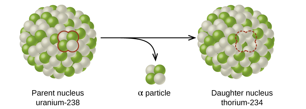
A quick word on the atomic representations used when discussing radioactive decay reactions. There are two numbers written to the left of the atomic symbol, for example, [latex]_{92}^{238}\text{U}[/latex]. The subscript, 92, denotes the atomic number of the element (number of protons); the superscript, 238, denotes the mass number of the isotope (number of protons + number of neutrons). [latex]_{92}^{235}\text{U}[/latex] is an isotope of [latex]_{92}^{238}\text{U}[/latex], and it also decarys via emission of an α particle, forming [latex]_{90}^{231}\text{Th}[/latex]. The subscripts and superscripts are necessary for balancing nuclear equations.
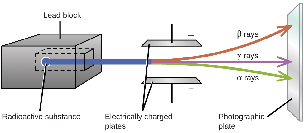
Ch9.12 Types of Radioactive Decay
Ernest Rutherford’s experiments involving the interaction of radiation with a magnetic or electric field (Figure 11) helped him determine that one type of radiation consisted of positively charged and relatively massive α particles; a second type consisted of negatively charged and much less massive β particles; and a third was uncharged electromagnetic waves, γ rays. Alpha particles ([latex]_2^4\text{He}[/latex], or [latex]_2^4{\alpha}[/latex]) are high-energy helium nuclei. Beta particles ([latex]_{-1}^0{\beta}[/latex], or [latex]_{-1}^0\text{e}[/latex]) are high-energy electrons, and gamma rays are photons of very high energy. Positrons ([latex]_{+1}^0\text{e}[/latex], or [latex]_{+1}^0{\beta}[/latex]) are positively charged electrons (“anti-electrons”). Note that for beta particles and positrons, which do not contain any protons, the subscript denotes the charge of the particle.
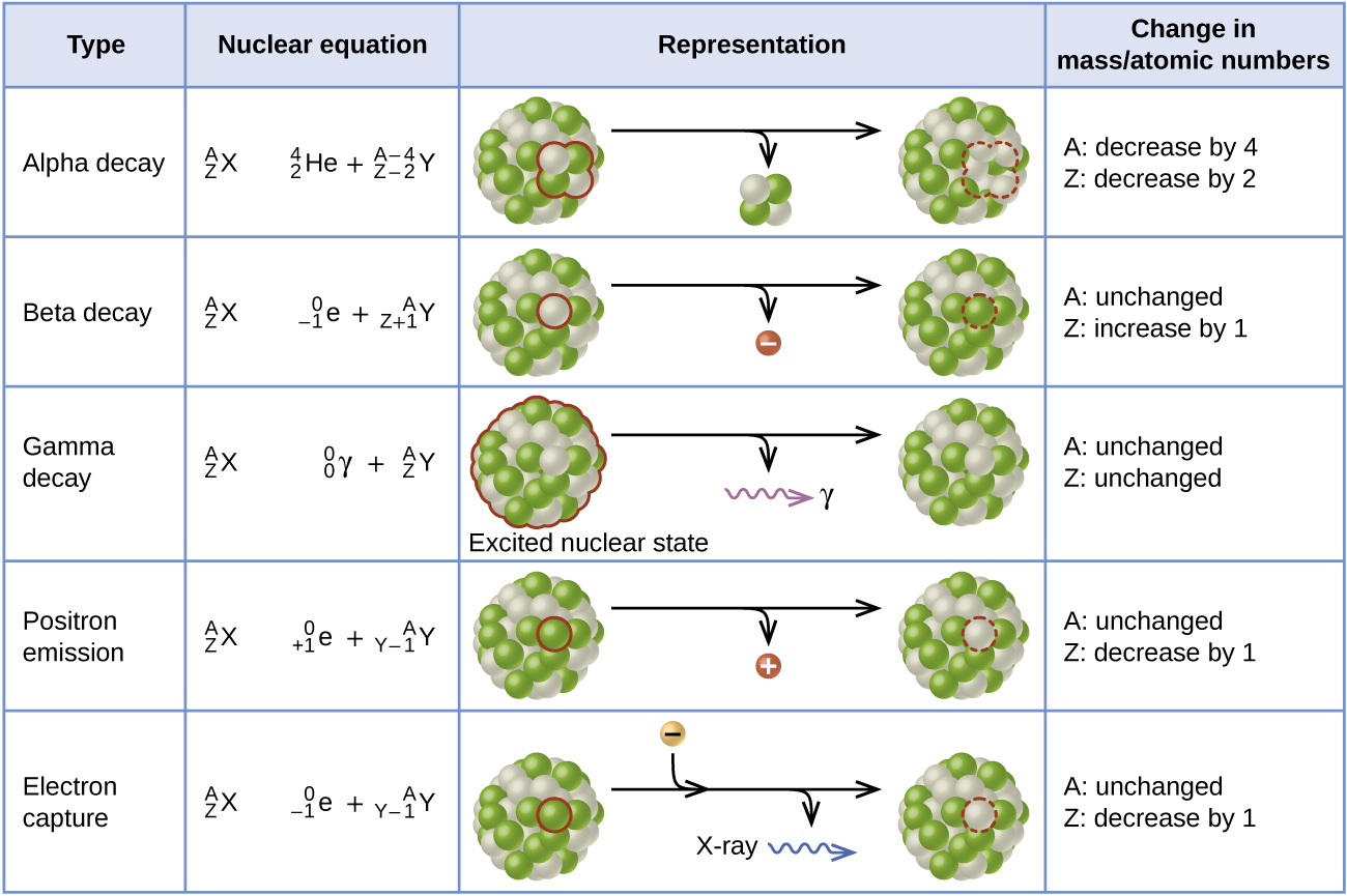
Alpha (α) decay is the emission of an α particle from the nucleus. For example, polonium-210 undergoes α decay:
Alpha decay occurs primarily in heavy nuclei (A > 200, Z > 83). The loss of an α particle gives a daughter nuclide with a mass number four units smaller and an atomic number two units smaller than those of the parent nuclide. Note that the sum of the subscript (proton numbers) on the product side is equal to the subscript on the reactant side. Same is true for the superscript (mass numbers) This reaction is balanced.
Beta (β) decay is the emission of an electron from a nucleus. Iodine-131 is an example of a nuclide that undergoes β decay:
Beta decay involves the conversion of a neutron into a proton and a β particle. The β particle (electron) emitted is from the atomic nucleus and is not one of the electrons surrounding the nucleus. Emission of a β particle does not change the mass number of the nuclide but does increase the number of its protons and decrease the number of its neutrons.
Gamma (γ) emission is observed when a nuclide decays via emission of a γ ray, a quantum of high-energy electromagnetic radiation. The energy of γ rays are quite high, in the range of keV to MeV (in comparison, x-rays have energies of 100 eV to 100 keV). Cobalt-60 is an example nuclide that decays via β emission as well as γ emission:
[latex]_{27}^{60}\text{Co}\;{\longrightarrow}\;_0^0{\gamma}\;+\;_{-1}^0{\beta}\;+\;_{28}^{60}\text{Ni}^*[/latex]
The presence of a nucleus in an excited state is often indicated by an asterisk (*). The excited Nickel-60 then decays to its ground state with the emission of γ radiation:
There is no change in mass number or atomic number during the emission of a γ ray unless the γ emission is accompanied by one of the other modes of decay.
Positron emission (β+ decay) is the emission of a positron from the nucleus. Oxygen-15 is an example of a nuclide that undergoes positron emission:
Positron decay is the conversion of a proton into a neutron with the emission of a positron.
Electron capture occurs when one of the inner electrons in an atom is captured by the atom’s nucleus, combines with a proton, transforming it into a neutron. For example, potassium-40 undergoes electron capture:
The loss of an inner shell electron leaves a vacancy that will be filled by one of the outer electrons. As the outer electron drops into the vacancy, it will emit energy. In most cases, the energy emitted will be in the form of an X-ray. Electron capture has the same effect on the nucleus as does positron emission: The atomic number is decreased by one and the mass number does not change. Whether electron capture or positron emission occurs is difficult to predict. The choice is primarily due to kinetic factors, with the one requiring the smaller activation energy being the one more likely to occur.
Figure 12 summarizes these types of decay.
PET Scan
Positron emission tomography (PET) scans use radiation to diagnose and track health conditions by revealing how parts of a patient’s body function (Figure 13). To perform a PET scan, a positron-emitting radioisotope is produced in a cyclotron and then attached to a substance that is used by the part of the body being investigated. This “tagged” compound, or radiotracer, is then put into the patient (injected via IV or breathed in as a gas), and how it is used by the tissue reveals how that organ or other area of the body functions.
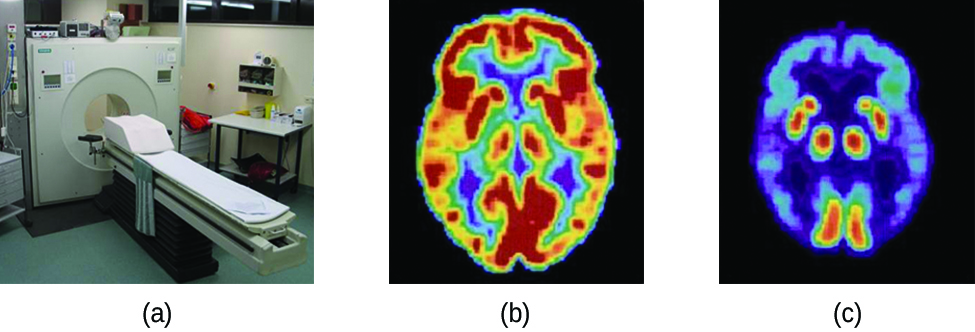
For example, F-18 is produced by proton bombardment of 18O ([latex]_8^{18}\text{O}\;+\;_1^1\text{p}\;{\longrightarrow}\;_9^{18}\text{F}\;+\;_0^1\text{n}[/latex]) and incorporated into a glucose analog called fludeoxyglucose (FDG). How FDG is used by the body provides critical diagnostic information. For example, since cancers use glucose differently than normal tissues, FDG can reveal presence of cancers. 18F emits positrons that interact with nearby electrons, producing a burst of gamma radiation. This energy is detected by the scanner and converted into a detailed, three-dimensional, color image that shows how that part of the patient’s body functions. Different levels of gamma radiation produce different amounts of brightness and colors in the image, which can then be interpreted by a radiologist to reveal what is going on. PET scans can detect heart damage and heart disease, help diagnose Alzheimer’s disease, indicate the part of a brain that is affected by epilepsy, reveal cancer, show what stage it is, and how much it has spread, and whether treatments are effective. Unlike magnetic resonance imaging (MRI) and X-rays, which only show how something looks, the big advantage of PET scans is that they show how something functions. PET scans are now usually performed in conjunction with a computed tomography scan.
Ch9.13 Half-Life of a Reaction
The half-life of a reaction (t1/2) is the time required for one-half of a given amount of reactant to be consumed. In each succeeding half-life, half of the remaining concentration of the reactant is consumed.
First-Order Reactions
We can derive an equation for determining the half-life of a first-order reaction from the integrated rate law as follows:
If we set the time t equal to the half-life, t1/2, the corresponding [A]t at this time is equal to one-half of its initial concentration, [latex][A]_{t_{1/2}} = \frac{1}{2}[A]_0[/latex]. Therefore:
Thus:
We can see that the half-life of a first-order reaction is inversely proportional to the rate constant k, and, conveniently, is independent of the concentration of the reactant. A fast reaction (shorter half-life) will have a larger k; a slow reaction (longer half-life) will have a smaller k.
Example 10
Calculation of a First-order Rate Constant using Half-Life
Calculate the rate constant for the first-order decomposition of hydrogen peroxide in water at 40 °C, using the data given in Figure 14.
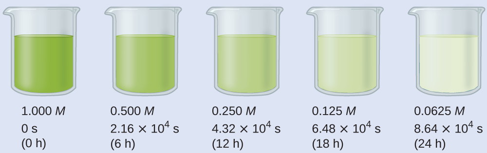
Solution
From the data in Figure 14, we see that it takes 6 hours for 1.000 M of H2O2 to decrease to 0.500 M, therefore the half-life for the decomposition of H2O2 is 2.16 × 10⁴ s. To find the rate constant:
Check Your Learning
The first-order radioactive decay of iodine-131 exhibits a rate constant of 0.138 d−1. What is the half-life for this decay?
Answer:
5.02 d.
Second-Order Reactions
We can derive the equation for calculating the half-life of a second order as follows:
When t = t1/2 and [latex][A]_{t_{1/2}} = \frac{1}{2}[A]_0[/latex]:
Thus:
For a second-order reaction, t1/2 is inversely proportional to the concentration of the reactant. This implies that the half-life is not constant throughout the reaction, and would increase as the reaction proceeds due to decreasing concentration of reactant. Consequently, we find the use of the half-life concept to be more complex for second-order reactions than for first-order reactions. Unlike with first-order reactions, the rate constant of a second-order reaction cannot be calculated directly from the half-life unless the initial concentration is known.
Zero-Order Reactions
We can derive an equation for calculating the half-life of a zero order reaction as follows:
When t = t1/2 and [latex][A]_{t_{1/2}} = \frac{1}{2}[A]_0[/latex]::
and
The half-life of a zero-order reaction decreases as the initial concentration decreases.
Equations for both differential and integrated rate laws and the corresponding half-lives for zero-, first-, and second-order reactions are summarized in Table 2.
| Zero-Order | First-Order | Second-Order | |
|---|---|---|---|
| rate law | rate = k | rate = k[A] | rate = k[A]2 |
| units of rate constant | M s−1 | s−1 | M−1 s−1 |
| integrated rate law | [A]t = −kt + [A]0 | ln[A]t = −kt + ln[A]0 | [latex]\frac{1}{[A]_t} = kt\;+\;(\frac{1}{[A]_0})[/latex] |
| plot needed for linear fit of rate data | [A] vs. t | ln[A] vs. t | [latex]\frac{1}{[A]}\;\text{vs.}\;t[/latex] |
| relationship between slope of linear plot and rate constant | k = −slope | k = −slope | k = +slope |
| half-life | [latex]t_{1/2} = \frac{[A]_0}{2k}[/latex] | [latex]t_{1/2} = \frac{0.693}{k}[/latex] | [latex]t_{1/2} = \frac{1}{[A]_0k}[/latex] |
| Table 2. Summary of Rate Laws for Zero-, First-, and Second-Order Reactions | |||
Ch9.14 Radioactive Half-Lives
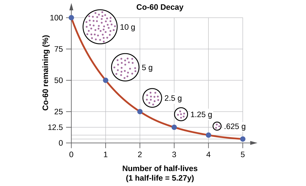
Radioactive decay follows first-order kinetics. Each radioactive nuclide has a characteristic, constant half-life (t1/2), the time required for half of the atoms in a sample to decay. An isotope’s half-life allows us to determine how long a sample of a useful isotope will be available, and how long a sample of an undesirable or dangerous isotope must be stored before it decays to a sufficiently low radiation level.
For example, cobalt-60, an isotope that emits gamma rays used to treat cancer, has a half-life of 5.27 years (Figure 15). In a given cobalt-60 source, since half of the [latex]_{27}^{60}\text{Co}[/latex] nuclei decay every 5.27 years, both the amount of material and the intensity of the radiation emitted is cut in half every 5.27 years. (Note that for a given substance, the intensity of radiation produced is directly proportional to the rate of decay of the substance and the amount of the substance.) This is as expected for a process following first-order kinetics. Thus, a cobalt-60 source that is used for cancer treatment must be replaced regularly to continue to be effective.
We can adapt the mathematical relationships used for first-order kinetics to describe nuclear decay. We generally substitute the number of nuclei, N, for the reactant concentration, and the decay constant, λ, for the rate constant. Hence, the rate for radioactive decay is:
decay rate = λN
If the decay rate is stated in nuclear decays per second, we refer to it as the activity of the radioactive sample.
It is possible to express the decay constant λ in terms of the half-life, t1/2:
The first-order equations relating amount, N, and time are:
where N0 is the initial number of nuclei or moles of the isotope, and Nt is the number of nuclei/moles remaining at time t.
Example 11
Rates of Radioactive Decay
[latex]_{27}^{60}\text{Co}[/latex] decays with a half-life of 5.27 years to produce [latex]_{28}^{60}\text{Ni}[/latex].
(a) What is the decay constant for the radioactive disintegration of cobalt-60?
(b) Calculate the fraction of a sample of the [latex]_{27}^{60}\text{Co}[/latex] isotope that will remain after 15.0 years.
(c) How long does it take for a sample of [latex]_{27}^{60}\text{Co}[/latex] to disintegrate to the extent that only 2.0% of the original amount remains?
Solution
(a) The value of the rate constant is given by:
(b) The fraction of [latex]_{27}^{60}\text{Co}[/latex] that is left after time t is given by [latex]\frac{N_t}{N_0}[/latex]. Rearranging the first-order relationship [latex]N_t = N_0e^{-{\lambda}t}[/latex] to solve for this ratio yields:
The fraction of [latex]_{27}^{60}\text{Co}[/latex] that will remain after 15.0 years is 0.138, or 13.8%.
(c) 2.00% of the original amount of [latex]_{27}^{60}\text{Co}[/latex] is equal to 0.0200×N0. Substituting this into the equation for time for first-order kinetics, we have:
Check Your Learning
Radon-222, [latex]_{86}^{222}\text{Rn}[/latex], has a half-life of 3.823 days. How long will it take for a sample of radon-222 with a mass of 0.750 g to decay, leaving only 0.100 g of radon-222?
Answer:
11.1 days
Because each nuclide has a specific number of nucleons, a particular balance of repulsion and attraction, and its own degree of stability, the half-lives of radioactive nuclides vary widely. For example: the half-life of [latex]_{83}^{209}\text{Bi}[/latex] is 1.9 × 10¹⁹ years; [latex]_{94}^{239}\text{Ra}[/latex] is 24,000 years; [latex]_{86}^{222}\text{Rn}[/latex] is 3.82 days; and element-111 (Rg for roentgenium) is 1.5 × 10⁻³ seconds.
Ch9.15 Radiometric Dating
Several radioisotopes have half-lives and other properties that make them useful for purposes of “dating” the origin of objects such as archaeological artifacts, formerly living organisms, or geological formations. This process is radiometric dating and has been responsible for many breakthrough scientific discoveries about the geological history of the earth, the evolution of life, and the history of human civilization. We will explore some of the most common types of radioactive dating and how the particular isotopes work for each type.
Radioactive Dating Using Carbon-14
The radioactivity of carbon-14 provides a method for dating objects that were a part of a living organism. This method of radiometric dating, which is also called radiocarbon dating or carbon-14 dating, can provide reasonably accurate dating of carbon-containing substances up to ~50,000 years old.
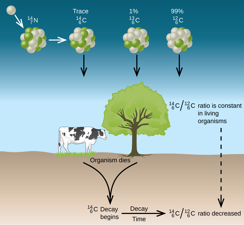
Naturally occurring carbon consists of three isotopes: [latex]_6^{12}\text{C}[/latex], which constitutes about 99% of the carbon on earth; [latex]_6^{13}\text{C}[/latex], about 1% of the total; and trace amounts of [latex]_6^{14}\text{C}[/latex]. Carbon-14 forms in the upper atmosphere by the reaction of nitrogen atoms with neutrons from cosmic rays:
All isotopes of carbon react with oxygen to produce CO2 molecules. The ratio of [latex]_6^{14}\text{CO}_2[/latex] to [latex]_6^{12}\text{CO}_2[/latex] depends on the ratio of [latex]_6^{14}\text{CO}[/latex] to [latex]_6^{12}\text{CO}[/latex] in the atmosphere. The natural abundance of [latex]_6^{14}\text{CO}[/latex] in the atmosphere is approximately 1 part per trillion; until recently, this has generally been constant over time, as seen is gas samples found trapped in ice. The incorporation of [latex]_6^{14}\text{CO}_2[/latex] and [latex]_6^{12}\text{CO}_2[/latex] into plants is a regular part of the photosynthesis process, which means that the 14C:12C ratio found in a living plant is the same as the 14C:12C ratio in the atmosphere. But when the plant dies, it no longer traps additional carbon through photosynthesis. Because 12C is a stable isotope and does not undergo radioactive decay, its concentration in the plant does not change. However, 14C decays by β emission with a half-life of 5730 years:
Thus, the 14C:12C ratio gradually decreases after the plant dies. The decrease in the ratio over time provides a measure of the time that has elapsed since the death of the plant (or other organism that ate the plant). Figure 16 visually depicts this process.
For example, if the 14C:12C ratio in a wooden object found in an archaeological dig is half what it is in a living tree, this indicates that the wooden object is 5730 years old. Highly accurate determinations of 14C:12C ratios can be obtained from very small samples (as little as a milligram) by the use of a mass spectrometer.
Example 12
Radiocarbon Dating
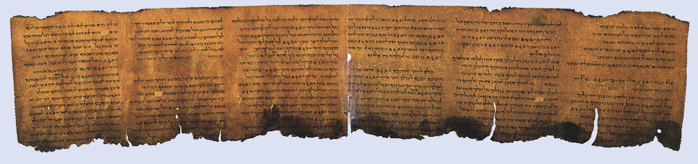
A tiny piece of paper (produced from formerly living plant matter) taken from the Dead Sea Scrolls has an activity of 10.8 disintegrations per minute per gram of carbon. If the initial 14C activity was 13.6 disintegrations/min/g of C, estimate the age of the Dead Sea Scrolls. (The half-life of 14C is 5730 years)
Solution
The activity, or rate of decay, is proportional to the amount of radioactive 14C left in the paper (decay rate = λN), so we can substitute the decay rates for the amount of 14C, N, in the relationship:
where the subscript 0 represents the time when the plants were cut to make the paper, and the subscript t represents the current time.
The decay constant can be determined from the half-life of 14C:
Substituting and solving, we have:
Therefore, the Dead Sea Scrolls are approximately 1900 years old (Figure 17).
Check Your Learning
More accurate dates of the reigns of ancient Egyptian pharaohs have been determined recently using plants that were preserved in their tombs. Samples of seeds and plant matter from King Tutankhamun’s tomb have a 14C decay rate of 9.07 disintegrations/min/g of C. How long ago did King Tut’s reign come to an end?
Answer:
about 3350 years ago, or approximately 1340 BC
The accuracy of a straightforward application of this technique depends on the 14C:12C ratio in a living plant being the same now as it was in an earlier era, but this is not always valid. For example, right now, due to the increasing accumulation of CO2 molecules, largely [latex]_6^{12}\text{CO}_2[/latex], in the atmosphere, caused by combustion of fossil fuels in which essentially all of the 14C has decayed, the 14C:12C ratio in our atmosphere is decreasing. This in turn affects the 14C:12C ratio in currently living organisms on the earth. Fortunately, we can use other data, such as tree dating via examination of annual growth rings, to calculate correction factors. With these correction factors, more accurate dates can be determined. In general, radioactive dating only works for about 10 half-lives; therefore, the limit for carbon-14 dating is about 57,000 years.
Radioactive Dating Using Nuclides Other than Carbon-14
Radioactive dating can also use other radioactive nuclides with longer half-lives to date older events. For example, uranium-238 (which decays in a series of steps into lead-206) can be used for establishing the age of rocks (and the approximate age of the oldest rocks on earth). Since 238U has a half-life of 4.5 billion years, it takes that amount of time for half of the original 238U to decay into 206Pb. In a sample of rock that does not contain appreciable amounts of 208Pb, the most abundant isotope of lead, we can assume that lead was not present when the rock was formed. Therefore, by measuring and analyzing the ratio of 238U:206Pb, we can determine the age of the rock, assumes that all of the 206Pb present came from the decay of 238U. If there is additional 206Pb present, which is indicated by the presence of other lead isotopes in the sample, it is necessary to make adjustments in the calculations. Potassium-argon dating uses a similar method. 40K decays by positron emission and electron capture to form 40Ar with a half-life of 1.25 billion years. If a rock sample is crushed and the amount of 40Ar gas that escapes is measured, determination of the 40Ar:40K ratio yields the age of the rock. Other methods, such as rubidium-strontium dating (87Rb decays into 87Sr with a half-life of 48.8 billion years), operate on the same principle. To estimate the lower limit for the earth’s age, scientists determine the age of various rocks and minerals, making the assumption that the earth is older than the oldest rocks and minerals in its crust. As of 2014, the oldest known rocks on earth are the Jack Hills zircons from Australia, found by uranium-lead dating to be almost 4.4 billion years old.
Example 13
Radioactive Dating of Rocks
An igneous rock contains 9.58 × 10⁻⁵ g of 238U and 2.51 × 10⁻⁵ g of 206Pb, and negligible amounts of 208Pb. Determine the approximate time at which the rock was formed. (238U decays into 206Pb with a half-life of 4.5 × 10⁹ y)
Solution
The sample of rock contains very little 208Pb, the most common isotope of lead, so we can safely assume that all the 206Pb in the rock was produced by the radioactive decay of 238U. When the rock was formed, it contained all of the 238U currently in it plus the 238U that has since undergone radioactive decay.
The amount of 238U currently in the rock is:
Because when one mole of 238U decays, it produces one mole of 206Pb, the amount of 238U that has undergone radioactive decay since the rock was formed is:
The total amount of 238U originally present in the rock is therefore:
The amount of time that has passed since the formation of the rock is given by:
with N0 representing the original amount of 238U and Nt representing the present amount of 238U.
The decay constant λ is:
Substituting and solving, we have:
Therefore, the rock is approximately 1.7 billion years old.
Check Your Learning
A sample of rock contains 6.14 × 10⁻⁴ g of 87Rb and 3.51 × 10⁻⁵ g of 87Sr. Calculate the age of the rock. (The half-life of the β decay of 87Rb is 4.7 × 10¹⁰ y.)
Answer:
3.7 × 10⁹ y
