
Additional Reading Materials
Chapter 13: Equilibrium
Ch13.1 Chemical Equilibrium
A chemical reaction is usually written in a way that suggests it proceeds in one direction, the direction in which we read, but all chemical reactions are reversible, and both the forward and reverse reaction occur to one degree or another depending on conditions. In a chemical equilibrium, the forward and reverse reactions occur at equal rates, and the concentrations of products and reactants remain constant. If we run a reaction in a closed system so that the products cannot escape, we often find the reaction does not yield 100% products. Instead, some reactants remain after the concentrations stop changing. At this point, when there is no further change in concentrations of reactants and products, we say the reaction is at equilibrium.
For example, when we place a sample of dinitrogen tetroxide (N2O4, a colorless gas) in a glass tube, it forms nitrogen dioxide (NO2, a brown gas) by the reaction
The color becomes darker as N2O4 is converted to NO2. When the system reaches equilibrium, both N2O4 and NO2 are present (Figure 1).
![A three-part diagram is shown. At the top of the diagram, three beakers are shown, and each one contains a sealed tube. The tube in the left beaker is full of a colorless gas which is connected to a zoom-in view of the particles in the tube by a downward-facing arrow. This particle view shows seven particles, each composed of two connected blue spheres. Each blue sphere is connected to two red spheres. The tube in the middle beaker is full of a light brown gas which is connected to a zoom-in view of the particles in the tube by a downward-facing arrow. This particle view shows nine particles, five of which are composed of two connected blue spheres. Each blue sphere is connected to two red spheres. The remaining four are composed of two red spheres connected to a blue sphere. The tube in the right beaker is full of a brown gas which is connected to a zoom-in view of the particles in the tube by a downward-facing arrow. This particle view shows eleven particles, three of which are composed of two connected blue spheres. Each blue sphere is connected to two red spheres. The remaining eight are composed of two red spheres connected to a blue sphere. At the bottom of the image are two graphs. The left graph has a y-axis labeled, “Concentration,” and an x-axis labeled, “Time.” A red line labeled, “N O subscript 2,” begins in the bottom left corner of the graph at a point labeled, “0,” and rises near the highest point on the y-axis before it levels off and becomes horizontal. A blue line labeled, “N subscript 2 O subscript 4,” begins near the highest point on the y-axis and drops below the midpoint of the y-axis before leveling off. The right graph has a y-axis labeled, “Rate,” and an x-axis labeled, “Time.” A red line labeled, “k subscript f, [ N subscript 2 O subscript 4 ],” begins in the bottom left corner of the graph at a point labeled, “0,” and rises near the middle of the y-axis before it levels off and becomes horizontal. A blue line labeled, “k subscript f, [ N O subscript 2 ] superscript 2,” begins near the highest point on the y-axis and drops to the same point on the y-axis as the red line before leveling off. The point where both lines become horizontal is labeled, “Equilibrium achieved.”](https://wisc.pb.unizin.org/app/uploads/sites/126/2017/08/CNX_Chem_13_01_equilibrium.jpg)
The formation of NO2 from N2O4 is a reversible reaction, which is identified by the equilibrium arrow (⇌). In a reversible reaction, the reactants can combine to form products and the products can react to form the reactants. Thus, not only can N2O4 decompose to form NO2, but the NO2 produced can react to form N2O4. As soon as the forward reaction produces any NO2, the reverse reaction begins and NO2 starts to react to form N2O4. At equilibrium, the concentrations of N2O4 and NO2 no longer change because the rate of NO2 formation is exactly equal to the rate of NO2 consumption, and the rate of formation of N2O4 is exactly equal to the rate of consumption of N2O4. Chemical equilibrium is a dynamic process: the numbers of reactant and product molecules remain constant, but there is a flux back and forth between them (Figure 2).
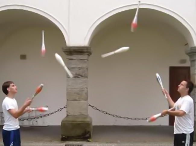
In a chemical equilibrium, the forward and reverse reactions do not stop, rather they continue to occur at the same rate, leading to constant concentrations of the reactants and the products. Plots showing how the reaction rates and concentrations change with respect to time are shown in Figure 1.
We can detect a state of equilibrium because the concentrations of reactants and products do not appear to change. However, it is important that we verify that the absence of change is due to equilibrium and not to a reaction rate that is so slow that changes in concentration are difficult to detect.
We use an equilibrium arrow when writing an equation for a reversible reaction. Such a reaction may or may not be at equilibrium. When we wish to speak about one particular component of a reversible reaction, we use a single arrow. For example, in the equilibrium shown in Figure 1, the rate of the forward reaction
is equal to the rate of the backward reaction
Equilibrium and Soft Drinks
The connection between chemistry and carbonated soft drinks goes back to 1767, when Joseph Priestley (1733–1804; mostly known today for his role in the discovery and identification of oxygen) discovered a method of infusing water with carbon dioxide to make carbonated water. In 1772, Priestly published a paper entitled “Impregnating Water with Fixed Air.” The paper describes dripping oil of vitriol (today we call this sulfuric acid, but what a great way to describe sulfuric acid: “oil of vitriol” literally means “liquid nastiness”) onto chalk (calcium carbonate). The resulting CO2 falls into the container of water beneath the vessel in which the initial reaction takes place; agitation helps the gaseous CO2 mix into the liquid water.
Carbon dioxide is slightly soluble in water. There is an equilibrium reaction that occurs as the carbon dioxide reacts with the water to form carbonic acid (H2CO3). Since carbonic acid is a weak acid, it can dissociate into protons (H+) and hydrogen carbonate ions [latex](\text{HCO}_3^{\;\;-})[/latex].
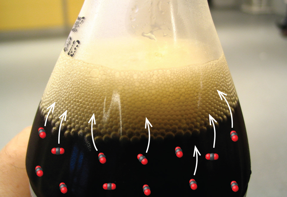
Today, CO2 can be pressurized into soft drinks, establishing the equilibrium shown above under a higher pressure condition. Once you open the beverage container, however, a cascade of equilibrium shifts occurs. First, the CO2 gas in the air space on top of the bottle escapes, causing the equilibrium between gas-phase CO2 and dissolved or aqueous CO2 to shift, lowering the concentration of CO2 in the soft drink. Less CO2 dissolved in the liquid leads to carbonic acid decomposing to dissolved CO2 and H2O. The lowered carbonic acid concentration causes a shift of the final equilibrium. The net result is that the CO2 bubbles up out of the beverage, releasing the gas into the air (Figure 3), results in a soft drink with a much lowered CO2 concentration, often referred to as “flat.”
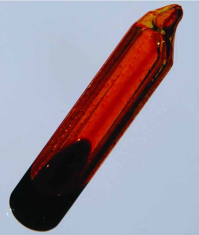
Let us consider the evaporation of bromine as a second example of a system at equilibrium.
An equilibrium can be established for a physical change—like this liquid to gas transition—as well as for a chemical reaction. Figure 4 shows a sample of liquid bromine at equilibrium with bromine vapor in a closed container. When we pour liquid bromine into an empty bottle in which there is no bromine vapor, some liquid evaporates: the amount of liquid decreases and the amount of vapor increases. If we cap the bottle so no vapor escapes, the amount of liquid and vapor will eventually stop changing and an equilibrium between the liquid and the vapor will be established. If the bottle were not capped, the bromine vapor would escape and no equilibrium would be reached.
Ch13.2 Equilibrium Constant
A general equation for a reversible reaction may be written as follows:
We can write the equilibrium constant (K) for this equation. When evaluated using concentrations, it is called Kc. We use brackets to indicate molar concentrations of reactants and products.
The equilibrium constant is equal to the molar concentrations of the products of the chemical equation (multiplied together) over the reactants (also multiplied together), with each concentration raised to the power of the coefficient of that substance in the balanced chemical equation.
Example 1
Evaluating an equilibrium constant
Gaseous nitrogen dioxide forms dinitrogen tetroxide according to this equation:
In a 1.0-L flask at 25 °C, the concentrations at equilibrium are [NO2] = 0.016 M and [N2O4] = 0.042 M. What is the value of the equilibrium constant for the reaction?
Solution
At equilibrium
[latex]K_c = \frac{[\text{N}_2\text{O}_4]}{[\text{NO}_2]^{2}} = \frac{0.042}{0.016^2} = 1.6\;\times\;10^{2}[/latex]
Note that dimensional analysis would suggest the unit for this Kc should be M−1. However, it is common practice to omit units for Kc values computed as described here, since it is the magnitude of an equilibrium constant that relays useful information. As will be discussed later, the rigorous approach to computing equilibrium constants uses dimensionless quantities derived from concentrations instead of actual concentrations, and so Kc values are truly unitless.
Check Your Learning
For the reaction [latex]2\text{SO}_2(g)\;+\;\text{O}_2(g)\;{\rightleftharpoons}\;2\text{SO}_3(g)[/latex], the concentrations at equilibrium are [SO2] = 0.90 M, [O2] = 0.35 M, and [SO3] = 1.1 M. What is the value of the equilibrium constant, Kc?
Answer:
Kc = 4.3
The magnitude of an equilibrium constant is a measure of the yield of a reaction when it reaches equilibrium. A large value for Kc indicates that equilibrium is attained after the reactants have been largely converted into products. A small value of Kc—much less than 1—indicates that equilibrium is attained when only a small proportion of the reactants have been converted into products.
Ch13.3 Working with Equilibrium Constants
In Example 5, it was mentioned that the common practice is to omit units when evaluating equilibrium constants. It should be pointed out that using concentrations in these computations is a convenient but simplified approach that sometimes leads to results that seemingly conflict with the law of mass action. For example, equilibria involving aqueous ions often exhibit equilibrium constants that vary quite significantly (are not constant) at high solution concentrations. This may be avoided by computing Kc values using the activities of the reactants and products in the equilibrium system instead of their concentrations. The activity of a substance is a measure of its effective concentration under specified conditions. While a detailed discussion of this important quantity is beyond the scope of an introductory text, it is necessary to be aware of a few important aspects:
- Activities are dimensionless (unitless) quantities and are in essence “adjusted” concentrations.
- For relatively dilute solutions, a substance’s activity and its molar concentration are roughly equal.
- Activities for pure condensed phases (solids and liquids) are equal to 1.
As a consequence of this last consideration, Kc expressions do not contain terms for solids or liquids (being numerically equal to 1, these terms have no effect on the expression’s value).
A homogeneous equilibrium is one in which all of the reactants and products are present in a single solution (by definition, a homogeneous mixture). Reactions between solutes in liquid solutions belong to one type of homogeneous equilibria. Several examples are provided here.
In each of these examples, the equilibrium system is an aqueous solution, as denoted by the aq annotations on the solute formulas. H2O(l) is the solvent for these solutions, its concentration does not appear as a term in the Kc expression, as discussed above, even though it may also appear as a reactant or product in the chemical equation.
A heterogeneous equilibrium is a system in which reactants and products are found in two or more phases. The phases may be any combination of solid, liquid, or gas phases, and solutions. Again, solids and pure liquids do not appear in equilibrium constant expressions (the activities of pure solids, pure liquids, and solvents are 1).
Some heterogeneous equilibria involve chemical changes; for example:
Other heterogeneous equilibria involve phase changes, for example, the evaporation of liquid bromine, as shown in the following equation:
The equilibrium constant expression must be manipulated if a reaction changes stoichiometry, is reversed or split into elementary steps.
When all the coefficients in a balanced chemical equation are multiplied by some factor n, then the new equilibrium constant is the original equilibrium constant raised to the nth power. For example:
When a reaction’s direction is reversed, the equilibrium constant for the new reaction is simply the inverse of that for the original reaction. For example:
When two reactions are added together to obtain a new reaction, the equilibrium constant for the new reaction is the product of the equilibrium constants for the original reactions. For example:
Ch13.4 Equilibrium Constant and Partial Pressure
Reactions in which all reactants and products are gases represent another class of homogeneous equilibria. We use molar concentrations in the following examples, but partial pressures of the gases may be used as well.
Note that the concentration of H2O(g) has been included in the last example because water is not the solvent in this gas-phase reaction and its concentration (and activity) changes.
Whenever gases are involved in a reaction, the partial pressure of each gas can be used instead of its concentration in the equation for the equilibrium constant because the partial pressure of a gas is directly proportional to its concentration at constant temperature. This relationship can be derived from the ideal gas equation, where M is the molar concentration of gas, [latex]\frac{n}{V}[/latex].
Thus, at constant temperature, the pressure of a gas is directly proportional to its concentration.
Using the partial pressures of the gases, we can write the equilibrium constant for the system [latex]\text{C}_2\text{H}_6(g)\;{\rightleftharpoons}\;\text{C}_2\text{H}_4(g)\;+\;\text{H}_2(g)[/latex] by following the same guidelines for deriving concentration-based expressions:
where KP designates an equilibrium constant derived using partial pressures instead of concentrations, [latex]P_{\text{C}_2\text{H}_6}[/latex] is the partial pressure of C2H6; [latex]P_{\text{H}_2}[/latex], the partial pressure of H2; and [latex]P_{\text{C}_2\text{H}_6}[/latex], the partial pressure of C2H4.
The equation relating Kc and KP is derived as follows. For the gas-phase reaction [latex]m\text{A}\;+\;n\text{B}\;{\rightleftharpoons}\;x\text{C}\;+\;y\text{D}[/latex]:
In this equation:
Δn is the difference between the sum of the coefficients of the gaseous products and the sum of the coefficients of the gaseous reactants in the reaction (the change in moles of gas between the reactants and the products). For the gas-phase reaction [latex]m\text{A}\;+\;n\text{B}\;{\leftrightharpoons}\;x\text{C}\;+\;y\text{D}[/latex], we have
Note that the gas constant, R, can be expressed in a variety of units with varying values corresponding to the unit conversions. Use the R value and associated units that match the partial pressure units used in the Kp expression. Oftentimes, the R used is 0.082057 [latex]\frac{\text{L}{\cdot}\text{atm}}{\text{mol}{\cdot}\text{K}}[/latex].
For heterogeneous equilibria that involve gases, equilibrium constants can also be expressed using partial pressures instead of concentrations. Two examples are:
Example 2
Calculation of KP
Write the equations for the conversion of Kc to KP for each of the following reactions:
(a) [latex]\text{C}_2\text{H}_6(g)\;{\rightleftharpoons}\;\text{C}_2\text{H}_4(g)\;+\;\text{H}_2(g)[/latex]
(b) [latex]\text{CO}(g)\;+\;\text{H}_2\text{O}(g)\;{\rightleftharpoons}\;\text{CO}_2(g)\;+\;\text{H}_2(g)[/latex]
(c) [latex]\text{N}_2(g)\;+\;3\text{H}_2(g)\;{\rightleftharpoons}\;2\text{NH}_3(g)[/latex]
(d) Kc is equal to 0.28 for the following reaction at 900 °C:
What is KP at this temperature?
Solution
(a) Δn = (2) − (1) = 1
KP = Kc (RT)Δn = Kc (RT)1 = Kc (RT)
(b) Δn = (2) − (2) = 0
KP = Kc (RT)Δn = Kc (RT)0 = Kc
(c) Δn = (2) − (1 + 3) = −2
KP = Kc (RT)Δn = Kc (RT)−2 = [latex]\frac{K_c}{(RT)^2}[/latex]
(d) KP = Kc (RT)Δn = (0.28)[(0.0821 [latex]\frac{\text{L}{\cdot}\text{atm}}{\text{mol}{\cdot}\text{K}}[/latex])(1173 K)]−2 = 3.0 × 10⁻⁵
Check Your Learning
Write the equations for the conversion of Kc to KP for each of the following reactions, which occur in the gas phase:
(a) [latex]2\text{SO}_2(g)\;+\;\text{O}_2(g)\;{\rightleftharpoons}\;2\text{SO}_3(g)[/latex]
(b) [latex]\text{N}_2\text{O}_4(g)\;{\rightleftharpoons}\;2\text{NO}_2(g)[/latex]
(c) [latex]\text{C}_3\text{H}_8(g)\;+\;5\text{O}_2(g)\;{\rightleftharpoons}\;3\text{CO}_2(g)\;+\;4\text{H}_2\text{O}(g)[/latex]
(d) At 227 °C, the following reaction has Kc = 0.0952:
What would be the value of KP at this temperature?
Answer:
(a) KP = Kc (RT)−1; (b) KP = Kc (RT); (c) KP = Kc (RT); (d) 160 or 1.6 × 10²
Ch13.5 Calculating Equilibrium Constants
Changes in concentrations or pressures of reactants and products occur as a reaction system approaches equilibrium. We can relate these changes to each other using the coefficients in the balanced chemical equation describing the system. We will use the decomposition of ammonia as an example. On heating, ammonia reversibly decomposes into nitrogen and hydrogen:
If a sample of ammonia decomposes in a closed system and the concentration of N2 increases by 0.11 M, the change in the N2 concentration, Δ[N2], the final concentration minus the initial concentration, is 0.11 M. The change is positive because the concentration of N2 increases.
The concentration of H2 also increases as ammonia decomposes. The balanced chemical equation tells us that Δ[H2] is three times Δ[N2] because for each mole of N2 produced, 3 moles of H2 are produced. Hence, Δ[H2] = 0.33 M.
The change in concentration of NH3, Δ[NH3], is twice that of Δ[N2]—2 moles of NH3 must decompose for each mole of N2 formed. However, the change in the NH3 concentration is negative because the concentration of ammonia decreases as it decomposes.
We can relate these relationships directly to the coefficients in the equation
Note that all the changes on one side of the arrows are of the same sign and that all the changes on the other side of the arrows are of the opposite sign.
If we did not know the magnitude of the change in the concentration of N2, we could represent it by the symbol x, Δ[N2] = x M. The changes in the other concentrations would then be represented as:
The simplest way for us to find the coefficients for the concentration changes in any reaction is to use the coefficients in the balanced chemical equation. The sign of the coefficient is positive when the concentration increases; it is negative when the concentration decreases.
Example 3
Determining Relative Changes in Concentration
Complete the changes in concentrations for each of the following reactions.
(a) [latex]\begin{array}{lcccc} \text{C}_2\text{H}_2(g) & + & 2\text{Br}_2(g) & {\rightleftharpoons} & \text{C}_2\text{H}_2\text{Br}_4(g) \\[0.5em] \;\;\; x & & \rule[0ex]{2.5em}{0.1ex} & & \rule[0ex]{2.5em}{0.1ex} \end{array}[/latex]
(b) [latex]\begin{array}{lcccc} \text{I}_2(aq) & + & \text{I}^{-}(aq) & {\rightleftharpoons} & \text{I}_3^{\;\;-}(aq) \\[0.5em] \rule[0ex]{2.5em}{0.1ex} & & \rule[0ex]{2.5em}{0.1ex} & & x \end{array}[/latex]
(c) [latex]\begin{array}{lcccccc} \text{C}_3\text{H}_8(g) & + & 5\text{O}_2(g) & {\rightleftharpoons} & 3\text{CO}_2(g) & + & 4\text{H}_2\text{O}(g) \\[0.5em] \;\;\; x & & \rule[0ex]{2.5em}{0.1ex} & & \rule[0ex]{2.5em}{0.1ex} & & \rule[0ex]{2.5em}{0.1ex} \end{array}[/latex]
Solution
(a) [latex]\begin{array}{lcccc} \text{C}_2\text{H}_2(g) & + & 2\text{Br}_2(g) & {\rightleftharpoons} & \text{C}_2\text{H}_2\text{Br}_4(g) \\[0.5em] \;\;\; x & & 2x & & -x \end{array}[/latex]
(b) [latex]\begin{array}{lcccc} \text{I}_2(aq) & + & \text{I}^{-}(aq) & {\rightleftharpoons} & \text{I}_3^{\;\;-}(aq) \\[0.5em] \;\; -x & & -x & & x \end{array}[/latex]
(c) [latex]\begin{array}{lcccccc} \text{C}_3\text{H}_8(g) & + & 5\text{O}_2(g) & {\rightleftharpoons} & 3\text{CO}_2(g) & + & 4\text{H}_2\text{O}(g) \\[0.5em] \;\;\; x & & 5x & & -3x & & -4x \end{array}[/latex]
Check Your Learning
Complete the changes in concentrations for each of the following reactions:
(a) [latex]\begin{array}{lcccc} 2\text{SO}_2(g) & + & \text{O}_2(g) & {\rightleftharpoons} & 2\text{SO}_3(g) \\[0.5em] \rule[0ex]{2.5em}{0.1ex} & & x & & \rule[0ex]{2.5em}{0.1ex} \end{array}[/latex]
(b) [latex]\begin{array}{lcc} \text{C}_4\text{H}_8(g) & {\rightleftharpoons} & 2\text{C}_2\text{H}_4(g) \\[0.5em] \rule[0ex]{2.5em}{0.1ex} & & -2x \end{array}[/latex]
(c) [latex]\begin{array}{lcccccc} 4\text{NH}_3(g) & + & 7\text{H}_2\text{O}(g) & {\rightleftharpoons} & 4\text{NO}_2(g) & + & 6\text{H}_2\text{O}(g) \\[0.5em] \rule[0ex]{2.5em}{0.1ex} & & \rule[0ex]{2.5em}{0.1ex} & & \rule[0ex]{2.5em}{0.1ex} & & \rule[0ex]{2.5em}{0.1ex} \end{array}[/latex]
Answer:
(a) 2x, x, −2x; (b) x, −2x; (c) 4x, 7x, −4x, −6x or −4x, −7x, 4x, 6x
Ch13.6 Calculation of an Equilibrium Constant
If concentrations of reactants and products at equilibrium are known, we can solve the equation for Kc, as it will be the only unknown.
The following example shows how to use the stoichiometry of the reaction and a combination of initial concentrations and equilibrium concentrations to determine an equilibrium constant. This technique, commonly called an ICE table—for Initial, Change, and Equilibrium–will be helpful in solving many equilibrium problems. A table is generated beginning with the equilibrium reaction in question. Underneath the reaction the initial concentrations of the reactants and products are listed—these conditions are usually provided in the problem and no shift toward equilibrium have happened yet. The next row of data is the change that occurs as the system shifts toward equilibrium—do not forget to consider the reaction stoichiometry as we’ve just described. The last row contains the concentrations once equilibrium has been reached.
Example 4
Calculation of an Equilibrium Constant
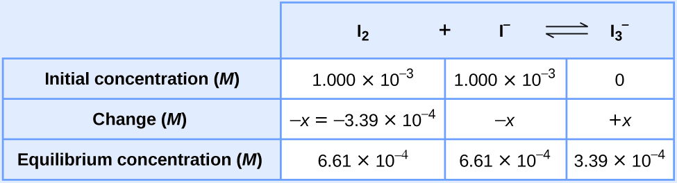
Iodine molecules react reversibly with iodide ions to produce triiodide ions.
If a solution starting with the concentrations of I2 and I− both equal to 1.000 × 10⁻³M and no triiodide ions, gives an equilibrium concentration of I2 of 6.61 × 10⁻⁴M, what is the equilibrium constant for the reaction?
Solution
We will begin this problem by calculating the changes in concentration as the system goes to equilibrium. Then we determine the equilibrium concentrations and, finally, the equilibrium constant. First, we set up an ICE table using −x as the change in concentration of I2.
![This table has two main columns and four rows. The first row for the first column does not have a heading and then has the following in the first column: Initial concentration ( M ), Change ( M ), Equilibrium concentration ( M ). The second column has the header, “I subscript 2 plus sign I superscript negative sign equilibrium arrow I subscript 3 superscript negative sign.” Under the second column is a subgroup of three rows and three columns. The first column has the following: 1.000 times 10 to the negative third power, negative x, [ I subscript 2 ] subscript i minus x. The second column has the following: 1.000 times 10 to the negative third power, negative x, [ I superscript negative sign ] subscript i minus x. The third column has the following: 0, positive x, [ I superscript negative sign ] subscript i plus x.](https://wisc.pb.unizin.org/app/uploads/sites/126/2017/08/CNX_Chem_13_04_ICETable1_img.jpg)
Since the equilibrium concentration of I2 is given as 6.61 × 10⁻⁴M, we can solve for x.
Now we can fill in the table with the concentrations at equilibrium.
We now calculate the value of the equilibrium constant.
Check Your Learning
Ethanol and acetic acid react and form water and ethyl acetate, the solvent responsible for the odor of some nail polish removers.
When 1 mol each of C2H5OH and CH3CO2H are allowed to react in 1 L of the solvent dioxane, equilibrium is established when 0.33 mol of each of the reactants remains. Calculate the equilibrium constant for the reaction. (Note: Water is a reactant, not a solvent, in this reaction. Also, be sure that the values in the ICE table have units of M, or mol/L.)
Answer:
Kc = 4
Ch13.7 Calculation of a Missing Equilibrium Concentration
If we know the equilibrium constant for a reaction and know the concentrations at equilibrium of all reactants and products except one, we can calculate the missing concentration.
Example 5
Calculation of a Missing Equilibrium Concentration
Nitrogen oxides are air pollutants produced by the reaction of nitrogen and oxygen at high temperatures. At 2000 °C, the value of the equilibrium constant for the reaction, [latex]\text{N}_2(g)\;+\;\text{O}_2(g)\;{\rightleftharpoons}\;2\text{NO}(g)[/latex], is Kc = 4.1 × 10⁻⁴. Find the concentration of NO(g) in an equilibrium mixture with air at 1 atm pressure at this temperature. In air, [N2] = 0.036 mol/L and [O2] 0.0089 mol/L.
Solution
We are given all of the equilibrium concentrations except that of NO. Thus, we can solve for the missing equilibrium concentration by rearranging the equation for the equilibrium constant.
Thus [NO] = 3.6 × 10⁻⁴ mol/L at equilibrium under these conditions.
Check Your Learning
The equilibrium constant for the reaction of nitrogen and hydrogen to produce ammonia at a certain temperature is 6.00 × 10⁻². Calculate the equilibrium concentration of ammonia if the equilibrium concentrations of nitrogen and hydrogen are 4.26 M and 2.09 M, respectively.
Answer:
1.53 mol/L
Ch13.8 Calculation of Changes in Concentration
If we know the equilibrium constant for a reaction and a set of concentrations of reactants and products that are not at equilibrium, we can calculate the changes in concentrations as the system comes to equilibrium, as well as the new concentrations at equilibrium. The typical procedure can be summarized in four steps.
- Balance the chemical reaction equation and determine the direction the reaction proceeds to come to equilibrium.
- Determine the relative changes needed to reach equilibrium—we typically represent the smallest change with the symbol x and express the other changes in terms of x, then write the equilibrium concentrations in terms of these changes.
- Substitute the equilibrium concentrations into the expression for the equilibrium constant, solve for x, and check any assumptions used to find x. Then calculate the equilibrium concentrations.
- Check the arithmetic by substituting the calculated equilibrium concentrations into the equilibrium expression and determining whether they give the equilibrium constant
Sometimes a particular step may be more complex in some problems and less complex in others. However, every calculation of equilibrium concentrations from a set of initial concentrations will involve these steps. An ICE table is useful in these calculations.
Example 6
Calculation of Concentration Changes as a Reaction Goes to Equilibrium
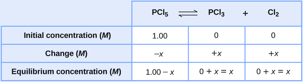
Under certain conditions, the equilibrium constant for the decomposition of PCl5(g) into PCl3(g) and Cl2(g) is Kc = 0.0211. What are the equilibrium concentrations of PCl5, PCl3, and Cl2 if the initial concentration of PCl5 was 1.00 M and there are no PCl3(g) and Cl2(g)?
Solution
Use the stepwise process described earlier.
- Determine the direction the reaction proceeds.
The balanced equation for the decomposition of PCl5 is
[latex]\text{PCl}_5(g)\;{\rightleftharpoons}\;\text{PCl}_3(g)\;+\;\text{Cl}_2(g)[/latex]Because we have no products initially, the reaction will proceed to the right.
- Determine the relative changes needed to reach equilibrium, then write the equilibrium concentrations in terms of these changes.
Let us represent the increase in concentration of PCl3 by the symbol x. The other changes may be written in terms of x by considering the coefficients in the chemical equation.
[latex]\begin{array}{lcccc} \text{PCl}_5(g) & {\rightleftharpoons} & \text{PCl}_3(g) & + & \text{Cl}_2(g) \\[0.5em] -x & & x & & x \end{array}[/latex]The changes in concentration and the expressions for the equilibrium concentrations are:
- Solve for x and the equilibrium concentrations.
Substituting the equilibrium concentrations into the equilibrium constant equation gives
[latex]K_c = \frac{[\text{PCl}_3][\text{Cl}_2]}{[\text{PCl}_5]} = \frac{(x)(x)}{(1.00\;-\;x)} = 0.0211[/latex]This equation contains only one variable, x, the change in concentration. We can write the equation as a quadratic equation:
[latex]0.0211 = \frac{(x)(x)}{(1.00\;-\;x)}[/latex][latex]0.0211(1.00\;-\;x) = x^2[/latex][latex]x^2\;+\;0.0211x\;-\;0.0211 = 0[/latex]and solve for x using the quadratic formula—an equation of the form ax2 + bx + c = 0 can be rearranged to solve for x:
[latex]x = \frac{-b\;{\pm}\;\sqrt{b^2\;-\;4ac}}{2a}[/latex]Here, a = 1, b = 0.0211, and c = −0.0211, which yields:
[latex]\begin{array}{r @{{}={}} l} x & \frac{-0.0211\;{\pm}\;\sqrt{(0.0211)^2\;-\;4(1)(-0.0211)}}{2(1)} \\[0.5em] & \frac{-0.0211\;{\pm}\;\sqrt{(4.45\;\times\;10^{-4})\;+\;(8.44\;\times\;10^{-2})}}{2} \\[0.5em] & \frac{-0.0211\;{\pm}\;0.291}{2} \end{array}[/latex]where
[latex]x = \frac{-0.0211\;+\;0.291}{2} = 0.135[/latex]or
[latex]x = \frac{-0.0211\;-\;0.291}{2} = -0.156[/latex]The second solution (x = −0.156) is physically impossible because we would end up with negative values for concentrations of the products at equilibrium. Thus, x = 0.135 M. (Quadratic equations often have two different solutions, and when calculating equilibrium constants, only one is physically possible.)
The equilibrium concentrations are
[latex][\text{PCl}_5] = 1.00\;M\;-\;0.135\;M = 0.87\;M[/latex][latex][\text{PCl}_3] = x = 0.135\;M[/latex][latex][\text{Cl}_2] = x = 0.135\;M[/latex] - Check the arithmetic.
Substitution into the expression for Kc (to check the calculation) gives
[latex]K_c = \frac{[\text{PCl}_3][\text{Cl}_2]}{[\text{PCl}_5]} = \frac{(0.135)(0.135)}{0.87} = 0.021[/latex]The equilibrium constant calculated from the equilibrium concentrations is equal to the value of Kc given in the problem (when rounded to the proper number of significant figures). Thus, the calculated equilibrium concentrations check.
Check Your Learning
Acetic acid, CH3CO2H, reacts with ethanol, C2H5OH, to form water and ethyl acetate, CH3CO2C2H5.
The equilibrium constant for this reaction with dioxane as a solvent is 4.0. What are the equilibrium concentrations when a mixture that is 0.15 M in CH3CO2H, 0.15 M in C2H5OH, 0.40 M in CH3CO2C2H5, and 0.40 M in H2O are mixed in enough dioxane to make 1.0 L of solution?
Answer:
[CH3CO2H] = 0.18 M, [C2H5OH] = 0.18 M, [CH3CO2C2H5] = 0.37 M, [H2O] = 0.37 M
Check Your Learning
A 1.00-L flask is filled with 1.00 moles of H2 and 2.00 moles of I2. The value of the equilibrium constant for the reaction of hydrogen and iodine reacting to form hydrogen iodide is 50.5 under the given conditions. What are the equilibrium concentrations of H2, I2, and HI in moles/L?
Answer:
[H2] = 0.065 M, [I2] = 1.06 M, [HI] = 1.87 M
Sometimes it is possible to find solutions to equilibrium problems without actually solving a quadratic (or more complicated) equation. First, however, it is useful to verify that equilibrium can be obtained starting from two extremes: all (or mostly) reactants and all (or mostly) products.
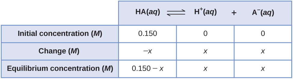
Consider the ionization of 0.150 M HA, a weak acid.
The most obvious way to determine the equilibrium concentrations would be to start with only reactants. This can be called the “all reactant” starting point. Using x for the amount of acid ionized at equilibrium, the ICE table is
Setting up and solving the quadratic equation gives
Using the positive (physically reasonable) root, the equilibrium concentrations are
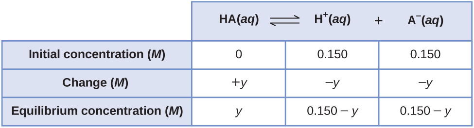
A less obvious way to solve the problem would be to assume all the HA ionizes first, and then the system comes to equilibrium. This can be called the “all product” starting point. Assuming all of the HA ionizes gives
Using these as initial concentrations and “y” to represent the concentration of HA at equilibrium, the ICE table is
Setting up and solving the quadratic equation gives
Retain a few extra significant figures to minimize rounding problems.
Rounding each solution to three significant figures gives
Using the physically significant root (0.140 M) gives the equilibrium concentrations as
Thus, the two approaches give the same results (to three decimal places), and show that both starting points lead to the same equilibrium conditions. The “all reactant” starting point resulted in a relatively small change (x) because the system was close to equilibrium, while the “all product” starting point had a relatively large change (y) that was nearly the size of the initial concentrations. It can be said that a system that starts “close” to equilibrium will require only a ”small” change in conditions (x) to reach equilibrium.
Recall that a small Kc means that very little of the reactants form products and a large Kc means that most of the reactants form products. If the system can be arranged so it starts “close” to equilibrium, then if the change (x) is small compared to any initial concentrations, it can be neglected. Small is usually defined as resulting in an error that does not change the answer given the significant figures involved. The following two examples demonstrate this.
Example 7
Approximate Solution Starting Close to Equilibrium
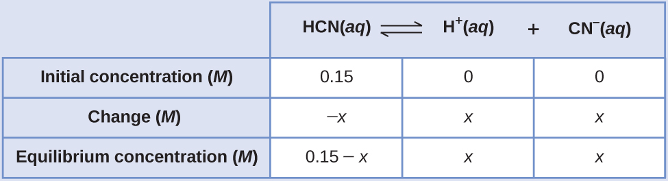
What are the concentrations at equilibrium of a 0.15 M solution of HCN?
Solution
Using “x” to represent the concentration of each product at equilibrium gives this ICE table.
The exact solution may be obtained using the quadratic formula with
solving
Thus [H+] = [CN–] = x = 8.6 × 10⁻⁶M and [HCN] = 0.15 – x = 0.15 M.
In this case, approximation can be used. From the equilibrium constant and the initial conditions, x is likely small compared to 0.15 M. More formally, if [latex]x\;{\ll}\;0.15[/latex], then 0.15 – x ≈ 0.15. If this assumption is true, then the equilibrium constant equation simplifies to
In this example, solving the exact quadratic equation and using approximations gave the same result to two significant figures. Additionally, plugging in the value of x shows that the 0.15 – x ≈ 0.15 approximation is indeed valid.
Check Your Learning
What are the equilibrium concentrations in a 0.25 M NH3 solution?
Assume that x is much less than 0.25 M.
Answer:
[latex][\text{OH}^{-}] = [\text{NH}_4^{\;\;+}] = 0.0021\;M[/latex]; [NH3] = 0.25 M
The second example requires that the original information be processed a bit, but it still can be solved using a small x approximation.
Example 8
Approximate Solution After Shifting Starting Concentration
Copper(II) ions form a complex ion in the presence of ammonia
If 0.010 mol Cu2+ is added to 1.00 L of a solution that has 1.00 M NH3, what are the concentrations when the system comes to equilibrium?
Solution
The initial concentration of copper(II) is 0.010 M. The equilibrium constant is very large so it would be better to start with as much product as possible because “all products” is much closer to equilibrium than “all reactants.” Note that Cu2+ is the limiting reactant; if all 0.010 M of it reacts to form product the concentrations would be
Using these “shifted” values as initial concentrations, with x as the free copper(II) ion concentration at equilibrium, the ICE table is
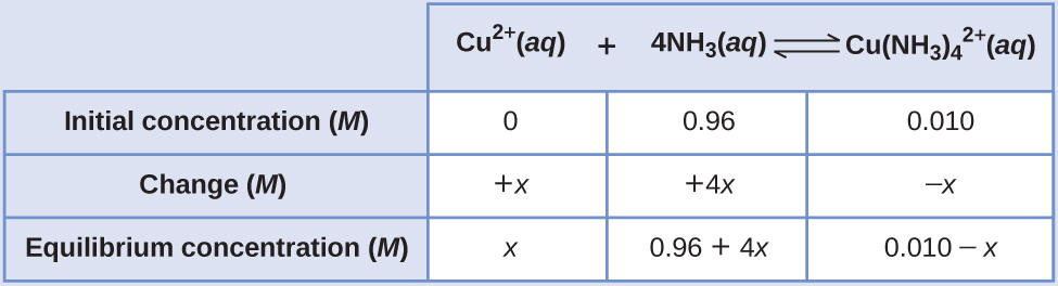
Since we are starting close to equilibrium, x should be small so that
This is much less than 0.96 M and 0.010 M, so the assumptions are valid. The concentrations at equilibrium are
By starting with the maximum amount of product, this system was near equilibrium and the change (x) was very small. With only a small change required to get to equilibrium, the equation for x was greatly simplified and gave a valid result well within the given significant figures.
Check Your Learning
What are the equilibrium concentrations when 0.25 mol Ni2+ is added to 1.00 L of 2.00 M NH3 solution?
With such a large equilibrium constant, first form as much product as possible, then assume that only a small amount (x) of the product shifts left.
Answer:
[latex][\text{Ni(NH}_3)_6^{\;\;2+}] = 0.25\;M[/latex], [NH3] = 0.50 M, [Ni2+] = 2.9 × 10⁻⁸M
Ch13.9 Reaction Quotient
We can write the reaction quotient (Q) for a generic reaction:
as (Qc is used to indicate usage of concentrations):
The numeric value of Qc for a given reaction depends on the concentrations of products and reactants present at the time when Qc is determined. When pure reactants are mixed, Qc = 0 because there are no products present at that point. As the reaction proceeds, the value of Qc increases as the concentrations of the products increase and the concentrations of the reactants decrease (Figure 5). When the reaction reaches equilibrium, the value of the reaction quotient no longer changes because the concentrations no longer change, and Qc = Kc.
![Three graphs are shown and labeled, “a,” “b,” and “c.” All three graphs have a vertical dotted line running through the middle labeled, “Equilibrium is reached.” The y-axis on graph a is labeled, “Concentration,” and the x-axis is labeled, “Time.” Three curves are plotted on graph a. The first is labeled, “[ S O subscript 2 ];” this line starts high on the y-axis, ends midway down the y-axis, has a steep initial slope and a more gradual slope as it approaches the far right on the x-axis. The second curve on this graph is labeled, “[ O subscript 2 ];” this line mimics the first except that it starts and ends about fifty percent lower on the y-axis. The third curve is the inverse of the first in shape and is labeled, “[ S O subscript 3 ].” The y-axis on graph b is labeled, “Concentration,” and the x-axis is labeled, “Time.” Three curves are plotted on graph b. The first is labeled, “[ S O subscript 2 ];” this line starts low on the y-axis, ends midway up the y-axis, has a steep initial slope and a more gradual slope as it approaches the far right on the x-axis. The second curve on this graph is labeled, “[ O subscript 2 ];” this line mimics the first except that it ends about fifty percent lower on the y-axis. The third curve is the inverse of the first in shape and is labeled, “[ S O subscript 3 ].” The y-axis on graph c is labeled, “Reaction Quotient,” and the x-axis is labeled, “Time.” A single curve is plotted on graph c. This curve begins at the bottom of the y-axis and rises steeply up near the top of the y-axis, then levels off into a horizontal line. The top point of this line is labeled, “k.”](https://wisc.pb.unizin.org/app/uploads/sites/126/2017/08/CNX_Chem_13_02_quotient.jpg)
That a reaction quotient always assumes the same value at equilibrium can be expressed as:
This equation is a mathematical statement of the law of mass action: When a reaction has attained equilibrium at a given temperature, the reaction quotient for the reaction always has the same value.
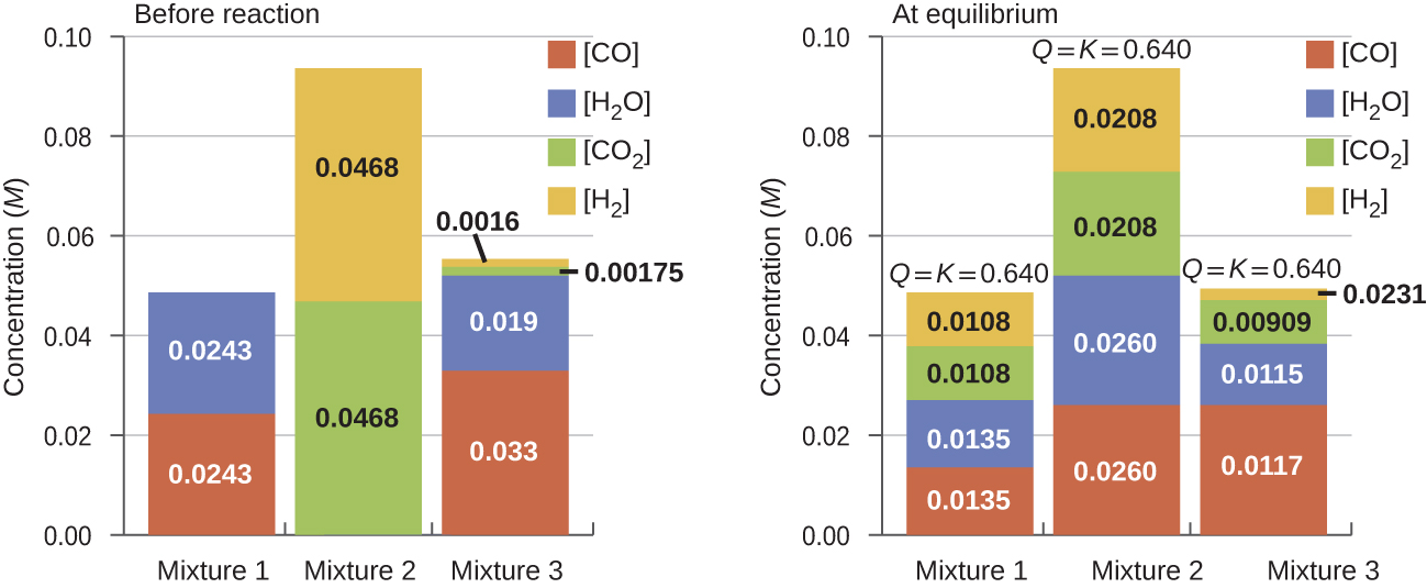
Once a value of Kc is known for a reaction, it can be used to predict directional shifts when compared to the value of Qc. A system that is not at equilibrium will proceed in the direction that establishes equilibrium. The data in Figure 6 illustrate this. When heated to a consistent temperature, 800 °C, different starting mixtures of CO, H2O, CO2, and H2 react to reach compositions adhering to the same equilibrium (the value of Qc changes until it equals the value of Kc).
It is important to recognize that an equilibrium can be established starting either from reactants or from products, or from a mixture of both. For example, equilibrium was established from Mixture 2 in Figure 6 when the products of the reaction were heated in a closed container. In fact, one technique to determine whether a reaction is truly at equilibrium is to start with only reactants in one experiment and start with only products in another. If the same value of the reaction quotient is observed when the concentrations stop changing in both experiments, then we may be certain that the system has reached equilibrium.
If we have a mixture of reactants and products that have not yet reached equilibrium, the changes necessary to reach equilibrium may not be obvious. In such a case, we can compare the values of Q and K for the system to predict the changes: when Qc < Kc, the reaction will proceed to the right (product side); when Qc > Kc, the reaction will proceed to the left (reactant side).
Example 9
Predicting the Direction of Reaction
Given here are the starting concentrations of reactants and products for three experiments involving the reaction:
Determine in which direction the reaction proceeds as it goes to equilibrium in each of the three experiments.
| Reactants/Products | Experiment 1 | Experiment 2 | Experiment 3 |
|---|---|---|---|
| [CO]initial | 0.0203 M | 0.011 M | 0.0094 M |
| [H2O]initial | 0.0203 M | 0.0011 M | 0.0025 M |
| [CO2]initial | 0.0040 M | 0.037 M | 0.0015 M |
| [H2]initial | 0.0040 M | 0.046 M | 0.0076 M |
Solution
Experiment 1:
Qc < Kc (0.039 < 0.64), the reaction will shift to the right.
Experiment 2:
Qc > Kc (140 > 0.64), the reaction will shift to the left.
Experiment 3:
Qc < Kc (0.49 < 0.64), the reaction will shift to the right.
Check Your Learning
Calculate the reaction quotient and determine the direction in which each of the following reactions will proceed to reach equilibrium.
(a) A 1.00-L flask containing 0.0500 mol of NO(g), 0.0155 mol of Cl2(g), and 0.500 mol of NOCl:
(b) A 5.0-L flask containing 17 g of NH3, 14 g of N2, and 12 g of H2:
(c) A 2.00-L flask containing 230 g of SO3(g):
Answer:
(a) Qc = 6.45 × 10³, shifts right. (b) Qc = 0.23, shifts left. (c) Qc = 0, shifts right.
