Lab 11: DATA ANALYSIS

During data analysis you will calculate the following:

1. The K_D for binding of DNSA to WT HCAII
2. The K_D for binding of DNSA to your HCAII mutant
3. The K_D for binding of AZ to WT HCAII
4. The K_D for binding of AZ to your HCAII mutant

For these calculations, you will use Excel to determine values and then plot ligand concentration versus fraction bound in Prism.

K_D for binding of DNSA to HCAII

Step 1: Look at your data. You should have fluorescence emission data at 470 nm (F₄₇₀) at various concentrations of DNSA that has been added to a solution containing HCAII. You should also have the volume of solution in each well, and the total concentration of DNSA ( [DNSA]_total) for each point in the titration. Identify any outliers in your data and determine whether they can be removed by applying the Dixon’s Q test.

For help with statistics, see the Appendix (link opens in a new tab): Appendix 2: Statistical methods used in 551 data analyses

The following video will help you become oriented to your data and show you how to identify and remove outliers.

For all videos, you should be able to actually read the numbers being shown. You may need to view full-screen, and/or manually increase the quality using the button in the lower right corner of the video. You can also turn on closed captioning for all videos.

Step 2: Correct the F₄₇₀ data for dilution during the titration (i.e. determine F_adjusted). Use the following equation:

Step 3: Calculate the fraction saturation, r, at each point (i.e. normalize the data). Use the following equation:

where F_min is the smallest value of F_adjusted and F_max is the largest value of F_adjusted.

Here is an example wt data set that has been analyzed through step 3. Note that the r values range from ~0 (at low DNSA) to ~1 (at high DNSA).

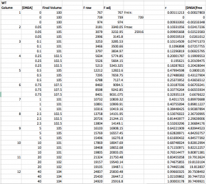
Step 4: Calculate the concentration of free DNSA at each point (i.e. calculate [DNSA]_free). Use the following equation:

The concentration of [HCAII]_total is probably 0.25 μM, unless you used something different.

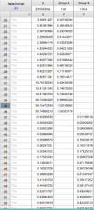
Step 5: Use Prism to plot r as a function of [DNSA]_free. Note that even though you did the experiment in triplicate, each Y-point (r) has a different X ([DNSA]_free), and so you cannot enter them as replicates in Prism. You can still enter all the data into Prism at once, you will just enter one “replicate” each for wt and mutant that contains all the data.

When you open Prism, choose “Enter and plot a single Y value for each point” from the initial menu. Enter the [DNSA]_free and r values for wt. Then add the mutant values below, always keeping [DNSA]_free in the “X” column but using two separate columns for r wt and r mutant.

See example:

The plot of your data should look hyperbolic, as is expected for ligand binding behavior.

See example plot:

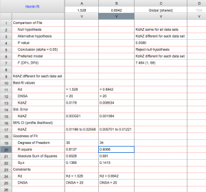
Fitting the equation should give you the K_D. You can also use Prism to determine whether there is statistical difference between wt and mutant. The following video demonstrates how to do the fit in Prism, which requires you to create your own fitting equation.

Note: the video uses an older version of Prism. In order to get error measurements in Prism 8 (and beyond), you need to follow the additional step: After choosing that you will compare Kd values, go to the “Confidence” tab. Select “Symmetrical (asymptotic) approximate CI” and then select “Show SE of parameters.”

K_D for binding of AZ to HCAII

 Much of this data processing is similar to what you just did for DNSA.

Step 1: As before, calculate the total volume of solution in each well after addition of ligand, as well as the total concentration of AZ ( [AZ]_total) for each point in the titration.

Step 2: Calculate F_adjusted as before, by identifying F_max and F_min and using the equation:

**Again, do this separately for wt and mutant (i.e. use different values for F_max and F_min).

Next calculate fraction saturation (r) as before using the equation:

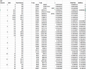
Step 3: Calculate the concentration of AZ-bound HCAII (i.e. [AZ*HCAII]) at each point. This should be a new column in your Excel sheet.

Since there is a negligible amount of protein not bound to either ligand, we approximate [HCAII]_free≈ 0.  Therefore, we can treat all non-fluorescing HCAII as AZ-bound, and thus use the equation:

Step 4: Calculate the concentration of free AZ at each point (i.e. calculate [AZ]_free].  Use the equation:

If you calculate any negative values for [AZ]_free, change them to 0.

Here is a sample data set that has been analyzed through step 4. Note that r values range from ~0 to ~1. Note also that a number of the [AZ]_free values, at the three lowest [AZ] tested, were actually negative and so were set to 0.

Step 5: Fit the data in Prism.

Open a new Prism file and, as before, choose “Enter and plot a single Y value for each point.” Copy your [AZ]_free values into the X column and r into the Y column – using separate columns for wt and mutant, just as before.

When you input your data into the data table, make the title of the column the K_D for DNSA that you measured in Part 1 above. So for example, instead of titling the column “wt” you might title it “1.568”. This looks a little weird, but will allow Prism to take the K_D for DNSA into account when you fit this data in the next steps.

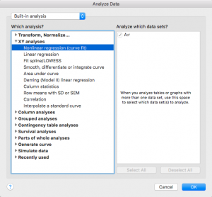
Click on “Analyze”

Select “XY Analyses” then “Nonlinear regression (curve fit)”

Press ok

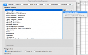
From the “+”drop down menu on the right side, choose “Create new equation”

(Note that if you are using Prism on a PC instead of a Mac this may look slightly different)

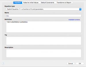
Give your equation a name

Type in the competitive langmuir isotherm equation:

Y=1/(1+(Kd/DNSA)(1+(x/(KdAZ))))

Note that in this equation “Kd” is the K_D for DNSA, which you determined in the first part of this analysis. “DNSA” is the concentration of DNSA that was used in this AZ experiment, probably 20 uM. “KdAZ” is the K_D for AZ, which you are going to have Prism find for you.

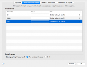
Now click on the “Rules for Initial Values” tab across the top. Remember that KdAZ is what we are having Prism solve for. In the drop down menu to the right of KdAZ, select *(Value of X at YMID)

Leave the other values alone.

Now click on the next tab over, “Default Constraints”

Remember that DNSA is a constant. Change the dropdown menu next to DNSA to “Constant equal to”

Kd is the K_D for DNSA that you measured in part 1, and that you made the column title in this data set. Change the dropdown menu to “Data set constant (from column title)”

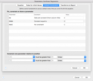
Press “ok”

You will get a dialogue box yelling at you for not defining rules. Just click “Continue”

Now your equation should show up under “User-defined equations”

With your equation highlighted, press ok

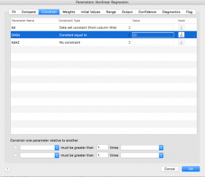
You will be taken to the “Constrain” tab, where you need to enter the concentration of DNSA that was used in your AZ experiment. Be sure you are consistent with your units here – I would use μM.

Next click over to the “Compare” tab. Select “Do the best-fit values of selected unshared parameters differ between data sets?”

Then select “KdAZ”.

Next click over to the “Confidence” tab and select the option to “Show SE of parameters.”

Finally, click “ok”!

Your data has been analyzed! It should look something like this sample data: