
Lab 9: DATA ANALYSIS
Your data will be provided by your TAs after you complete the in-lab activities.
During data analysis you will perform these major steps:
- Blank and normalize your fluorescence data
- Fit the data directly in GraphPad Prism to determine:
- the ΔGunfolding
- the CM
- Manually manipulate the fluorescence data to create two plots:
- fraction of folded protein (Xf) vs. [urea]
- ΔGunfolding vs. [urea]
Part 1: Blank and normalize your fluorescence data
- The following video helps get you oriented to your data and demonstrates how to average your blanks and subtract them from your experimental values. NOTE: For all videos, you should be able to actually read the numbers being shown. You may need to view full-screen, and/or manually increase the video quality. You can also turn on closed captioning for all videos.
- NOTE: The urea concentrations tested are included in the “Setup” page of the data file. These may not be the same concentrations you were planning to use! Be sure to take the urea concentrations from the data file, not from your plan.
- For each protein (wt and mutant), create plots that overlay the emission spectrum of your protein at each urea concentration, as demonstrated in the following video.
- The plate reader records values in relative fluorescence units (RFU), which depend on the instrument settings. All samples should have the same protein concentration, but pipetting errors can cause slight (or large) variances. Therefore, it is helpful to normalize the data, using the fluorescence at a wavelength that is not very affected by the state of the protein (340 nm) as a reference point. First, look at the plots you created in step 2 and be sure the folded curves have a peak around 324 nm, while the unfolded curves shift to higher wavelengths. If not, talk to the teaching staff before proceeding with the data analysis.
- Normalize the data by calculating the ratio between two emissions: 324/340. 324 nm is the point where you should observe a peak in the folded protein curves. 340 nm is the approximate point where all the curves come closest to intersecting.
- Discard data from any wells that appear to have no (or too little) protein. These would appear as approximately a straight line in the fluorescence vs wavelength plot, and/or give a negative or otherwise unreasonable 324/340 ratio. DO NOT use data from these wells in any of the remaining analyses.
Part 2: Fit the data directly in Prism to determine the ΔGunfolding and CM
- This video walks through the basics of fitting data in Prism. Download the sample data file so that you can follow along with the video. Sample file can be downloaded from Canvas here: Sample Lab 9 Data Analysis File
- PLEASE NOTE: This video was made using Prism 7 for Mac. Your version may differ slightly.
- The first thing you need to do is download the correct fitting equation from the sample data file. Unfortunately you can’t directly download a Prism equation, but this is a workaround:
- Open the sample file and navigate to the “Nonlinear fit of…” page under the “Results” heading.
- Look for the cell with a blue link “Nonlin fit” in the top left corner of the sheet. Click on this link.
- Without changing any parameters, click “OK”
- Your computer has now run the analysis and downloaded the correct fitting equation into your Prism. You can now close the sample data file.
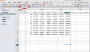
- Open a new project file in Prism and select “Enter 3 replicate values in side-by-side subcolumns,” hit “Create”

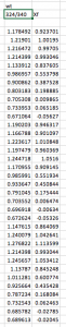
- Paste the urea concentrations used on the X column and the calculated 324/340 emission ratio values for wild type on the “Group A” columns and for mutant on the “Group B” columns. Rename the titles.
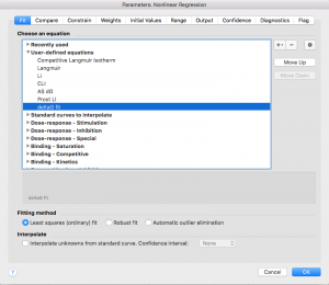
- Analyze the data using the “Analyze” button. Select “Nonlinear regression (curve fit)” under “XY analyses”
- Under both “Recently used” and “User-defined equations” you should see the equation from the sample data: “deltaG fit Prism9”. Select this equation but DO NOT click “OK” yet.
Mathematical Description of the ΔGunfolding Fit
Determining the ΔGunfolding depends on the linear relationship between [urea] and deltaG.:
As discussed in lecture, there is a logarithmic relationship between the ΔGunfolding and the fraction folded (Xf), meaning a plot of [urea] vs Xf is sigmoidal:
ΔGunfolding = -RT ln Keq
and Keq is related to Xf because:
Keq = [U] / [F]
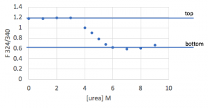
Going back one step further, the fluorescence data you just entered into Prism is also sigmoidal, but is spread between a “top” value (fluorescence representing fully folded protein) and “bottom” (fully unfolded) rather than between 1 and 0.
Since we know the mathematical relationships relating these plots, we can combine them to derive a function that relates the normalized fluorescence directly to ΔGunfolding. This equation is shown below, and is what you will fit in Prism:

where x is [urea],
bottom and top are fits of the bottom and top baselines for the sigmoidal curve,
a is the slope of the linear relationship between [urea] and deltaG,
0.59 is used as the value of RT, and
dGo is the ΔGunfolding value to be determined from the fit.
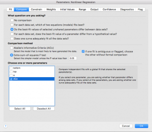
- Click on the “Compare” tab and select “Do the best-fit values of selected unshared parameters differ between data sets?” Then choose “dGo”. This will force Prism to do a t-test to compare your wild type and mutant results (see appendix for more information on statistics).
- Error reporting has changed slightly in the new version of Prism. Click on the “Confidence” tab. In older versions, you were able to check box a for “Show SE of parameters.” In order to select this option in the newest Prism, you have to first select “Symmetrical (asymptotic) approximate CI” then select “Show SE of parameters.” If you are not able to show standard error in your version of Prism, that is ok. You can check “Calculate CI of parameters” using the option “Asymmetrical CI” instead.
- Note: Prism doesn’t recommend fitting this way, but Standard Error values are useful for us. Based on a few initial trials, this type of CI calculation only differs very slightly from the recommended type.
- Now press OK.
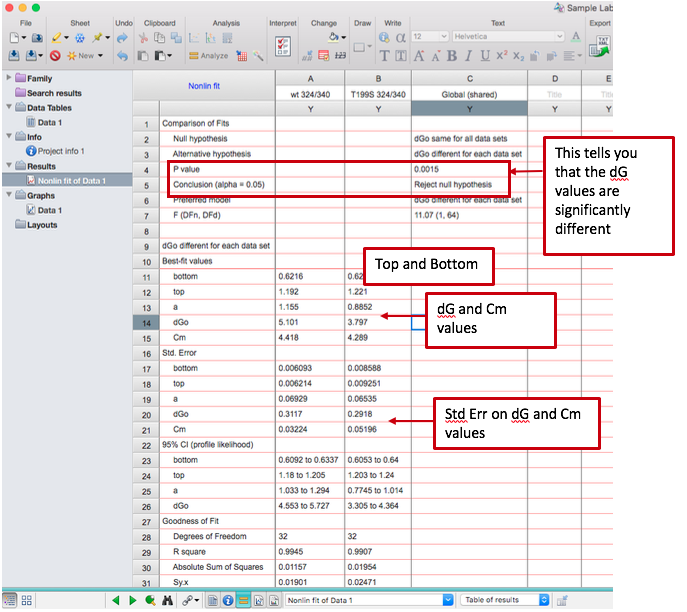
- The program will run a fit of your data according to the equation as described above. You are interested in the parameters “dGo” and “Cm” in the output. You will also see 95% confidence values and/or standard error values for the dGo and Cm; you should report those.
- Prism will also tell you whether or not the dGo (ΔGunfolding) is statistically different for the two data sets, including a p-value. You should also report this.
- Note that what Prism runs this analysis, it does it in two ways: allowing the values for wt and mutant to be different, and forcing them to be the same. Even if Prism determines that the p-value is high and the values are therefore not statistically significant, you should report the values from the analysis where the two were allowed to be different (i.e. don’t report the exact same value for wt and mutant).
- Under “Best-fit values,” you are also given a “Top” and “Bottom.” Note each of these values for both wt and mutant – you will need them in the next step of the data analysis.
Example output (note that depending on your version of Prism, there may or may not be standard error reported):
Part 3: Manually manipulate the fluorescence data and create plots of interest
The following analyses can all be completed in Excel. You will manually approximate the same fit that you just ran in Prism, by calculating the Xf and then the ΔGunfolding values for your data set. Doing so will help you assess the quality of your data, and allow you to create useful plots to include in your lab report.
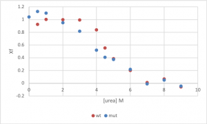
- Return to your fluorescence ratios, and further normalize this data by calculating the fraction of folded protein Xf at each urea concentration. This will essentially spread the data between 1 (fully folded, which corresponds to the points near 0M urea) and 0 (fully unfolded, which corresponds to the points at very high urea concentrations).
- Calculate Xf for each data point, using the experimental emission ratio at each urea concentration. Do this calculation separately for wt and mutant, as they probably have different top and bottom values.
Xf = (Experimental fluorescence ratio – Bottom) / (Top – Bottom)
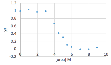
- Plot Xf against urea concentration, including both wt and mutant on the same graph.
Sample data:
- The next step is to determine the ΔGunfolding from the fraction folded (Xf) at each urea concentration, using the following equations:
Keq = (Xf)-1 – 1
ΔGunfolding = –RT ln(Keq)
Use RT values to give units of kcal/mol. Omit any data points where Keq<0.
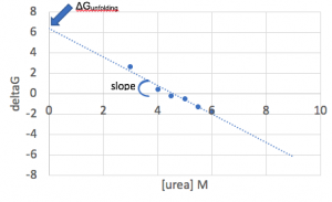
- Create a plot of the ΔGunfolding vs [urea]. Notice that increasing the urea concentration favors unfolding (reduction in ΔGunfolding) and that ΔGunfolding becomes zero and eventually negative, as shown below.
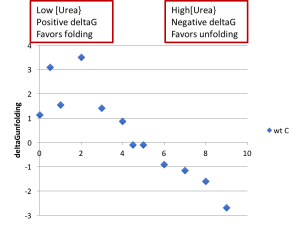
- With an ideal data set, you would be able to fit the linear region of this plot, and the y-intercept of that fit line would match the ΔGunfolding value from the Prism fit. However, in practice, large amounts of error where Xf is either small or large make this sort of fit unreliable.
