
M7Q3: Emission Spectra and H Atom Levels
Introduction
The 19th century quest by scientists to explain the phenomena of line spectra led to a further break from the classical theory of physics and a step toward the development of quantum mechanics. This section will explore the discoveries of the era which explained observations of our natural world, such as, Why do objects have color? This section includes worked examples, sample problems, and a glossary.
Learning Objectives for Emission Spectra and H atom levels
- Summarize the connection between discrete line spectra and how energy levels of atoms are quantized.
| Emission Line Spectra | - Predict the observed emission and absorption frequencies and wavelengths of photons using the Bohr theory.
| Hydrogen Atom Levels |
| Key Concepts and Summary | Key Equations | Glossary | End of Section Exercises |
Emission Line Spectra
Another paradox within the classical electromagnetic theory that scientists in the late nineteenth century struggled with concerned the light emitted from atoms and molecules. As seen in the previous section, when solids, liquids, or condensed gases are heated sufficiently, they radiate some of the excess energy as light. Photons produced in this manner have a range of energies, and thereby produce a continuous spectrum in which an unbroken series of wavelengths is present. Most of the light generated from stars (including our sun) is produced in this fashion. You can see all the visible wavelengths of light present in sunlight by using a prism to separate them. As can be seen in the continuous spectrum (Figure 1, top), sunlight also contains UV light (shorter wavelengths) and IR light (longer wavelengths) that can be detected using instruments but that are invisible to the human eye. Incandescent (glowing) solids such as tungsten filaments in incandescent lights also give off light that contains all wavelengths of visible light. These continuous spectra can often be approximated by blackbody radiation curves at some appropriate temperature.
In contrast to continuous spectra, light can also occur as discrete or line spectra having very narrow line widths interspersed throughout the spectral regions such as those shown in Figure 1, bottom. Each emission line consists of a single wavelength of light, which implies that the light emitted by a gas consists of a set of discrete energies. For example, when an electric discharge passes through a tube containing hydrogen gas at low pressure, the H2 molecules are broken apart into separate H atoms and we see a blue-pink color. Passing the light through a prism produces a line spectrum, indicating that this light is composed of photons of four visible wavelengths, as shown in Figure 1.
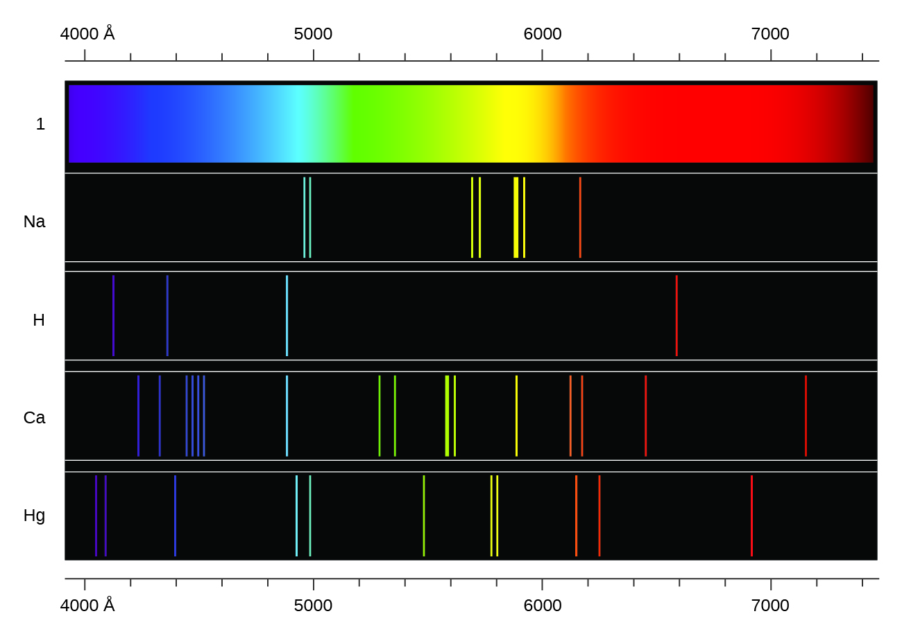
Exciting a gas at low partial pressure using an electrical current, or heating it, will produce line spectra. Fluorescent light bulbs and neon signs operate in this way (Figure 2). Each element displays its own characteristic set of lines, as do molecules, although their spectra are generally much more complicated.

The origin of discrete spectra in atoms and molecules was extremely puzzling to scientists in the late nineteenth century, since according to classical electromagnetic theory, only continuous spectra should be observed. Even more puzzling, in 1885, Johann Balmer was able to derive an empirical equation that related the four visible wavelengths of light emitted by hydrogen atoms to whole integers. That equation is the following one, in which k is a constant:
 = k
= k , n = 3, 4, 5, 6
Other discrete lines for the hydrogen atom were found in the UV and IR regions. Johannes Rydberg generalized Balmer’s work and developed an empirical formula that predicted all of hydrogen’s emission lines, not just those restricted to the visible range, where, n1 and n2 are integers, n1 < n2, and R∞ is the Rydberg constant (1.097 × 10⁷ m−1).
= R∞
Even in the late nineteenth century, spectroscopy was a very precise science, and so the wavelengths of light emitted from a hydrogen atom were measured to very high accuracy, which implied that the Rydberg constant could be determined very precisely as well. That such a formula as simple as the Rydberg formula could account for such precise measurements seemed astounding at the time, but it was the eventual explanation for emission spectra by Neils Bohr in 1913 that ultimately convinced scientists to abandon classical physics and spurred the development of modern quantum mechanics.
Hydrogen Atom Levels
Following the work of Ernest Rutherford and his colleagues in the early twentieth century, the picture of atoms consisting of tiny dense nuclei surrounded by lighter and even tinier electrons continually moving about the nucleus was well established. This picture was called the planetary model, since it pictured the atom as a miniature “solar system” with the electrons orbiting the nucleus like planets orbiting the sun. The simplest atom is hydrogen, consisting of a single proton as the nucleus about which a single electron moves. This classical mechanics description of the atom is incomplete, however, since an electron moving in an elliptical orbit would be accelerating (by changing direction) and, according to classical electromagnetism, it should continuously emit electromagnetic radiation. This loss in orbital energy should result in the electron’s orbit getting continually smaller until it spirals into the nucleus, implying that atoms are inherently unstable.
In 1913, Niels Bohr attempted to resolve the atomic paradox by ignoring classical electromagnetism’s prediction that the orbiting electron in hydrogen would continuously emit light. Instead, he incorporated Planck’s ideas of quantization and Einstein’s finding that light consists of photons whose energy is proportional to their frequency into the classical mechanics description of the atom. Bohr assumed that the electron orbiting the nucleus would not normally emit any radiation (the stationary state hypothesis), but it would emit or absorb a photon if it moved to a different orbit. The energy absorbed or emitted would reflect differences in the orbital energies according to this equation:
|ΔE| = |Ef – Ei| = hν = 
In this equation, h is Planck’s constant and Ei and Ef are the initial and final orbital energies, respectively. The absolute value of the energy difference is used, since frequencies and wavelengths are always positive. Instead of allowing for continuous values for the angular momentum, energy, and orbit radius, Bohr assumed that only discrete values for these could occur (actually, quantizing any one of these would imply that the other two are also quantized). Bohr’s expression for the quantized energies of energy level n for the H atom is:
En =  , n = 1, 2, 3, …
In this expression, A is a constant comprising fundamental constants such as the electron mass and charge and Planck’s constant, Z is the atomic number for H which is 1, and n is the energy level. When Bohr calculated his theoretical value for the Rydberg constant, R∞, and compared it with the experimentally accepted value, he got excellent agreement, where A = 2.179 × 10⁻¹⁸ J. Since the Rydberg constant was one of the most precisely measured constants at that time, this level of agreement was astonishing and meant that Bohr’s model was taken seriously, despite the many assumptions that Bohr needed to derive it.
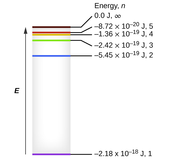
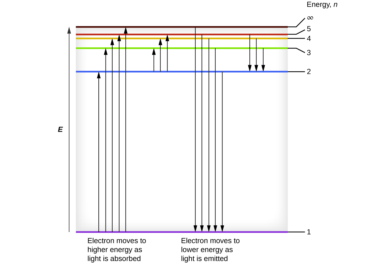
The lowest few energy levels of hydrogen are shown in Figure 3. One of the fundamental laws of physics is that matter is most stable with the lowest possible energy. Thus, the electron in a hydrogen atom usually moves in the n = 1 orbit, the orbit in which it has the lowest (most negative) energy. When the electron is in this lowest energy orbit, the atom is said to be in its ground electronic state (or simply ground state). If the atom receives energy from an outside source, it is possible for the electron to move to an orbit with a higher n value and the atom is now in an excited electronic state (or simply an excited state) with a higher energy. When an electron transitions from an excited state (higher energy orbit) to a less excited state, or ground state, the difference in energy is emitted as a photon. The emitted photon has an energy equal to the difference in energy between the two levels. Similarly, if a photon is absorbed by an atom, the energy of the photon must match an energy difference between two levels in the atom to move an electron from a lower energy orbit to a higher energy one.
We can relate the energy of electrons in atoms to what we learned previously about energy. The law of conservation of energy says that we can neither create nor destroy energy. Thus, if a certain amount of external energy is required to excite an electron from one energy level to another, that same amount of energy will be liberated when the electron returns to its initial state (Figure 4). In effect, an atom can “store” energy by using it to promote an electron to a state with a higher energy and release it when the electron returns to a lower state. The energy can be released as one quantum of energy (i.e., one photon), as the electron returns to its ground state (say, from n = 5 to n = 1), or it can be released as two or more smaller quanta (i.e., more than one photon) as the electron falls to an intermediate state, then to the ground state (say, from n = 5 to n = 4, emitting one quantum, then to n = 1, emitting a second quantum). The energy differences between these levels will be equal to the energy of the photon emitted when the electron relaxes to the ground state (or required to excite the electron to an excited state). Recall that the energy of the photon is related to the frequency of light according to the equation E = hν. Therefore, the frequency of emitted light can provide information about the energy level transitions in an atom. For example, take the line spectra in Figure 1. We can first determine the frequency of the different lines. These frequencies can be used to calculate energies. These energies correspond to discrete energy level transitions within the atom.
Any electron transition, ΔE, can be expressed if the initial energy level (ni) and final energy level (nf) are known:
ΔE = Efinal – Einitial
ΔE = -2.179 × 10⁻¹⁸  J
J
As the electron’s energy increases (as n increases), the electron is found at greater distances from the nucleus (r increases). As we saw at the beginning of the semester, the Coulomb potential is the attractive force between the negatively and positively charged particles. In this case, the Coulomb potential describes the attractive force between the positively charged nucleus and the negatively charged electron. As n increases, therefore, the distance from the nucleus also increases due to the inverse dependence on distance in the Coulomb potential: As the electron moves away from the nucleus, the electrostatic attraction between it and the nucleus decreases, and it is held less tightly in the atom. Note that as n gets larger and the orbits get larger, their energies get closer to zero (less negative energies), and so the limits n → ∞ and r → ∞ imply that E = 0 corresponds to the ionization limit where the electron is completely removed from the nucleus and the neutral atom becomes an ion. Thus, for hydrogen in the ground state n = 1, the ionization energy would be:
ΔE = Efinal – Einitial
ΔE = -2.179 × 10⁻¹⁸  J
J
With three extremely puzzling paradoxes now solved (the photoelectric effect, blackbody radiation, and the hydrogen atom), and all involving Planck’s constant in a fundamental manner, it became clear to most physicists at that time that the classical theories that worked so well in the macroscopic world were fundamentally flawed and could not be extended down into the microscopic domain of atoms and molecules. Unfortunately, despite Bohr’s remarkable achievement in deriving a theoretical expression for the Rydberg constant, he was unable to extend his theory to the next simplest atom, He, which has only two electrons. Bohr’s model was severely flawed, since it was still based on the classical mechanics notion of precise orbits, a concept that was later found to be untenable in the microscopic domain. As a result, the quantum mechanical model was developed and superseded classical mechanics.
Bohr’s model of the hydrogen atom provides insight into the behavior of matter at the microscopic level, but it is does not account for electron–electron interactions in atoms with more than one electron. It does introduce several important features of all models used to describe the distribution of electrons in an atom. These features include the following:
- The energies of electrons (energy levels) in an atom are quantized, described by quantum numbers: discrete numbers having only specific allowed values and used to characterize the arrangement of electrons in an atom.
- An electron’s energy increases with increasing distance from the nucleus.
- The discrete energies (lines) in the spectra of the elements result from quantized electronic energies.
Of these features, the most important is the postulate of quantized energy levels for an electron in an atom. As a consequence, the model laid the foundation for the quantum mechanical model of the atom. Bohr won a Nobel Prize in Physics for his contributions to our understanding of the structure of atoms and how that is related to line spectra emissions.
Example 1
Calculating the Energy of an Electron in a Bohr Orbit
Early researchers were very excited when they were able to predict the energy of an electron at a particular distance from the nucleus in a hydrogen atom. If a spark promotes the electron in a hydrogen atom into an orbit with n = 3, what is the calculated energy, in joules, of the electron?
Solution
The energy of the electron is given by this equation:
E = –
The atomic number, Z, of hydrogen is 1; A = 2.179 × 10⁻¹⁸ J; and the electron is characterized by an n value of 3. Thus,
E =  = -2.421 × 10⁻¹⁹ J
Check Your Learning
The electron is promoted even further to an orbit with n = 6. What is its new energy?
Answer:
−6.053 × 10⁻²⁰ J
Example 2
Calculating the Energy and Wavelength of Electron Transitions in a One–electron (Bohr) System
What is the energy (in joules) and the wavelength (in meters) of the line in the spectrum of hydrogen that represents the movement of an electron from Bohr orbit with n = 4 to the orbit with n = 6? In what part of the electromagnetic spectrum do we find this radiation?
Solution
In this case, the electron starts out with n = 4, so n1 = 4. It comes to rest in the n = 6 orbit, so n2 = 6. The difference in energy between the two states is given by this expression:
ΔE = E1 – E2 = 2.179 × 10⁻¹⁸  J = 2.179 × 10⁻¹⁸
  J
J
ΔE = 2.179 × 10⁻¹⁸  J = 7.566 × 10⁻²⁰ J
This energy difference is positive, indicating a photon enters the system (is absorbed) to excite the electron from the n = 4 orbit up to the n = 6 orbit. It is always a good idea to think double check yourself at this stage and make sure that the sign for ΔE that you calculate makes sense with the direction the electron is moving: if the electron is moving to a higher energy level, ΔE should be positive. The wavelength of a photon with this energy is found by the expression E = . Rearrangement gives:
λ =  = (6.626 × 10⁻³⁴ J·s) ×
  = 2.626 × 10⁻⁶ m
We can see that this wavelength is found in the infrared portion of the electromagnetic spectrum.
Check Your Learning
What is the energy in joules and the wavelength in meters of the photon produced when an electron falls from the n = 5 to the n = 3 level in a He+ ion (Z = 2 for He+)?
Answer:
6.198 × 10⁻¹⁹ J; 3.205 × 10⁻⁷ m (note that the change in energy for the electron for this transition, ΔE, is negative since the electron is moving from n = 5 to n = 3, but the energy of the photon is always positive.)
Key Concepts and Summary
Bohr incorporated Planck’s and Einstein’s quantization ideas into a model of the hydrogen atom that resolved the paradox of atom stability and discrete spectra. The Bohr model of the hydrogen atom explains the connection between the quantization of photons and the quantized emission from atoms. Bohr described the hydrogen atom in terms of an electron moving in a circular orbit about a nucleus. He postulated that the electron was restricted to certain orbits characterized by discrete energies. Transitions between these allowed orbits result in the absorption or emission of photons. When an electron moves from a higher-energy orbit to a more stable (lower-energy) one, energy is emitted in the form of a photon. To move an electron from a ground state to a more excited one, a photon of energy must be absorbed. Using the Bohr model, we can calculate the energy of an electron and the radius of its orbit in any one-electron system.
Key Equations
- ΔE = AZ2
- ΔE = Efinal – Einitial = -2.179 × 10⁻¹⁸ J
Glossary
- Bohr’s model of the hydrogen atom
- structural model in which an electron moves around the nucleus only in circular orbits, each with a specific allowed radius; the orbiting electron does not normally emit electromagnetic radiation, but does so when changing from one orbit to another.
- continuous spectrum
- electromagnetic radiation given off in an unbroken series of wavelengths (e.g., white light from the sun)
- excited state
- state having an energy greater than the ground-state energy
- ground state
- state in which the electrons in an atom, ion, or molecule have the lowest energy possible
- line spectrum
- electromagnetic radiation emitted at discrete wavelengths by a specific atom (or atoms) in an excited state
- quantization
- occurring only in specific discrete values, not continuous
- quantum number
- integer number having only specific allowed values and used to characterize the arrangement of electrons in an atom
Chemistry End of Section Exercises
- How are the Bohr model and the Rutherford model of the atom similar? How are they different?
- Using the Bohr model, determine the energy, in joules, necessary to ionize a ground-state hydrogen atom.
- The electron volt (eV) is a convenient unit of energy for expressing atomic-scale energies. It is the amount of energy that an electron gains when subjected to a potential of 1 volt; 1 eV = 1.602 × 10⁻¹⁹ J. Using the Bohr model, determine the energy, in electron volts, of the photon produced when an electron in a hydrogen atom moves from the orbit with n = 5 to the orbit with n = 2.
- Using the Bohr model, determine the lowest possible energy for the electron in the He+ ion.
- Using the Bohr model, determine the energy of an electron with n = 8 in a hydrogen atom.
- Using the Bohr model, determine the energy in joules of the photon produced when an electron in a He+ ion moves from the orbit with n = 5 to the orbit with n = 2.
- Using the Bohr model, determine the energy in joules of the photon produced when an electron in a Li2+ ion moves from the orbit with n = 2 to the orbit with n = 1.
- Consider a large number of hydrogen atoms with electrons randomly distributed in the n = 1, 2, 3, and 4 orbits.
- How many different wavelengths of light are emitted by these atoms as the electrons fall into lower-energy orbitals?
- Calculate the lowest and highest energies of light produced by the transitions described in part (a).
- Calculate the frequencies and wavelengths of the light produced by the transitions described in part (b).
- The following questions refer to an electron that transitions from energy levels n=4 to n=2 in the hydrogen atom.
- Is the transition going to absorb or emit a photon?
- Use Figure 3 to determine the change in energy for this transition. Be sure to include the + or – sign.
- Determine the wavelength of light (in nanometers) corresponding to the energy change calculated in part (b).
- The energy level diagram for a hydrogen atom is shown below. The arrows represent electron transitions between two energy levels. Which of the transitions would result in the absorption of a photon with the shortest wavelength?
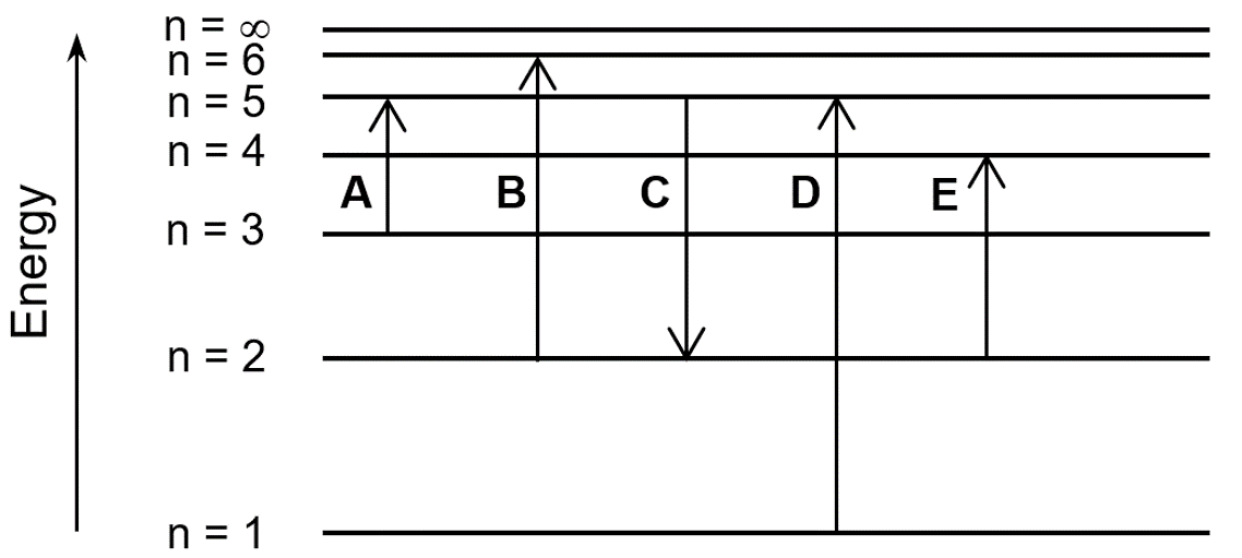
- The diagram below shows the Bohr model of the hydrogen atom.

- Which arrow indicates the absorption of a photon with the longest wavelength?
- Which arrow corresponds a transition between the ground state and the first excited state of hydrogen?
Answers to Chemistry End of Section Exercises
- Both involve a relatively heavy nucleus with electrons moving around it, although strictly speaking, the Bohr model works only for one-electron atoms or ions. According to classical mechanics, the Rutherford model predicts a miniature “solar system” with electrons moving about the nucleus in circular or elliptical orbits that are confined to planes. If the requirements of classical electromagnetic theory that electrons in such orbits would emit electromagnetic radiation are ignored, such atoms would be stable, having constant energy and angular momentum, but would not emit any visible light (contrary to observation). If classical electromagnetic theory is applied, then the Rutherford atom would emit electromagnetic radiation of continually increasing frequency (contrary to the observed discrete spectra), thereby losing energy until the atom collapsed in an absurdly short time (contrary to the observed long-term stability of atoms). The Bohr model retains the classical mechanics view of circular orbits confined to planes having constant energy and angular momentum, but restricts these to quantized values dependent on a single quantum number, n. The orbiting electron in Bohr’s model is assumed not to emit any electromagnetic radiation while moving about the nucleus in its stationary orbits, but the atom can emit or absorb electromagnetic radiation when the electron changes from one orbit to another. Because of the quantized orbits, such “quantum jumps” will produce discrete spectra, in agreement with observations.
- 2.179 × 10⁻¹⁸ J
- 2.856 eV (4.576 × 10⁻¹⁹ J)
- -8.716 × 10⁻¹⁸ J
- -3.405 × 10⁻²⁰ J
- 1.830 × 10⁻¹⁸ J
- 1.471 × 10⁻¹⁷ J
- (a) 6
(b) En=4→n=1 = 2.043 × 10⁻¹⁸ J, En=4→n=3 = 1.059 × 10⁻¹⁹ J
(c) n=4→n=1: ν = 3.083 × 10¹⁵, λ = 97.24 nm; n=4→n=3: ν = 1.599 × 10¹⁴, λ = 1,875 nm - (a) emit a photon; (b) -4.09 × 10⁻¹⁹ J; (c) 486 nm
- D
- (a) E; (b) B
Please use this form to report any inconsistencies, errors, or other things you would like to change about this page. We appreciate your comments. 🙂
