
M13Q4: Introduction to Flooding Techniques and Experimental Use of Initial Rates
Learning Objectives
- Apply the experimental technique of flooding to reactions involving more than one reactant to determine reaction orders, the rate constant (k), and the rate law for a reaction.
- Evaluate experimental data using the method of initial rates to determine reaction orders, the rate constant, and the rate law for a reaction.
Experimental Use of the Initial Rates Method When Only One Reactant is Present
The method of initial rates can be used experimentally by running a reaction, such as A → product, with different starting concentrations of A and measuring how the concentration of A decreases over time. The resulting data can be plotted as seen in Figure 1.
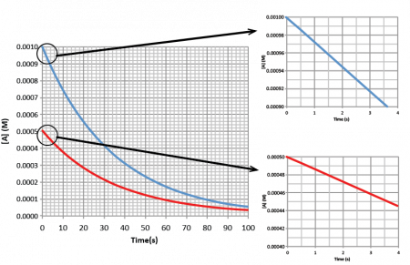
Experimental data from monitoring the decomposition of A in the reaction A → product, when the initial concentration of A is 0.0010 M and 0.0005 M, as shown in the left graph of Figure 1. The smaller graphs, made by graphing only the first few data points in the larger graph, allow one to calculate the initial rate of each reaction by finding the change of concentration over the change in time at the very beginning of the reaction. The absolute value of the slope of these graphs are the initial rates of reaction (recall that the rates of reaction are always a positive value). For [A] = 0.0010 M, the initial rate of reaction is 2.90 × 10⁻⁵ M/s and for [A] = 0.0005 M, the initial rate of reaction is 1.45 × 10⁻⁵ M/s.
Doubling the concentration of A results in a doubling of the rate of reaction so the reaction is first-order with respect to A and the rate law is:
rate = k[A]
Experimental Use of Initial Rates When Two or More Reactants Are Present; The Flooding Method
However, many reactions involve two or more reactants—how can we find the reaction order and rate constants experimentally for these reactions? We can use the “flooding” method, where one reactant is at a much larger concentration than the other, making the larger concentration reactant appear to have a constant concentration with respect to the change that occurs with the smaller concentration reactant.
Let’s consider the reaction:
A + B → Products
where
rate = k[A]m[B]n
To isolate the effect of reactant A on the reaction rate, we can run the reaction under a large excess of reactant B, i.e., flooding the reaction mixture with B so that A is the limiting reagent. The concentration of reactant B remains effectively constant during the reaction because the change in the concentration of B is so small that it is considered negligible.
By varying the larger reactant concentrations versus time, we can use the initial rates of reaction to determine the reaction order with respect to reactants A and B.
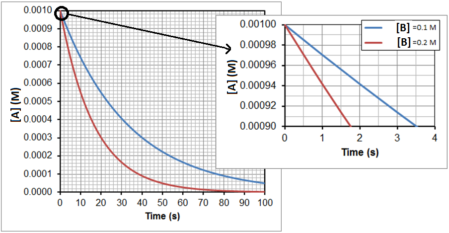
In Figure 2, two experimental runs are plotted, where the initial concentration of A is 0.0010 M each time, but the initial concentration of B is 0.1 M in one run, shown in blue, and 0.2 M in the other, shown in red. Zooming in on the first few seconds, as shown in the smaller graph, allows for the calculation of the initial rates. The resulting data is shown in table below:
| Trial | [A] (M) | [B] (M) | Initial Rate (M/s) |
| 1 | 0.0010 | 0.10 | 2.9 x 10⁻⁵ |
| 2 | 0.0010 | 0.20 | 5.7 x 10⁻⁵ |
Now we will do the same experiment again, varying the initial concentration of A from trial 1 to trial 3 but holding the initial concentration of B constant for both trials. The results can be seen in Figure 3.
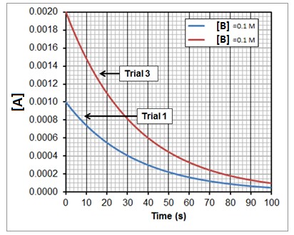
After finding the initial rate for each trial as we did before, we can expand the data table to include all 3 trials:
| Trial | [A] (M) | [B] (M) | Initial Rate (M/s) |
| 1 | 0.0010 | 0.10 | 2.9 x 10⁻⁵ |
| 2 | 0.0010 | 0.20 | 5.7 x 10⁻⁵ |
| 3 | 0.0020 | 0.10 | 5.7 x 10⁻⁵ |
Now there is enough data to find the rate law. When [A] is held constant and [B] is doubled, the rate doubles so the reaction is first-order with respect to B. Additionally, when [B] is held constant but [A] is doubled, the rate doubles so the reaction is first-order with respect to A. This gives a rate law of:
rate = k[A][B]
Key Concepts and Summary
Using the method of initial rates, either from a table or the slope on a graph, is useful for any chemical reaction. But when there are two or more reactants, completing enough experiments to calculate the order of each reactant can be tedious. Instead, the method of flooding can be utilized, where one reactant is at a much higher concentration than the other. We will see soon that by plotting the concentration of the lower concentration, or limiting, reactant, we can calculate the order of the lower concentration reactant. And by analyzing the slope in the first few time points of the higher concentration reactant, we can calculate the order of the higher concentration reactant.
Glossary
- flooding
- a method used when there are two or more reactants, where one reactant is at a much larger concentration than the other, making the larger concentration reactant appear to have a constant concentration with respect to the change that occurs in the smaller concentration reactant
Please use this form to report any inconsistencies, errors, or other things you would like to change about this page. We appreciate your comments. 🙂
