M13Q5: Integrated Rate Laws; Application of Pseudo-First Order (Flooding) Techniques

Chem 103 Textbook Team; Chem 104 Textbook Team

M13Q5: Integrated Rate Laws; Application of Pseudo-First Order (Flooding) Techniques

Learning Objectives

Given the initial concentration of a reactant, use integrated rate laws to determine the concentration of reactant after a given time has passed or how long it will take for the reactant to reach a certain concentration.
| First Order | Second Order | Zero Order |
Apply the experimental technique of flooding to reactions involving more than one reactant to determine reaction orders, the observed rate constant (k_obs), the rate constant (k), and the rate law for a reaction.
| Flooding |
Evaluate experimental data using the integrated rate law method to determine reaction orders, the rate constant, and the rate law for a reaction.

Integrated Rate Laws

The rate laws we have seen so far relate the rate and the concentrations of reactants. We can also determine a second form of each rate law that relates the concentrations of reactants and time. These are called integrated rate laws. We can use an integrated rate law to determine the amount of reactant or product present after a period of time or to estimate the time required for a reaction to proceed to a certain extent. For example, an integrated rate law is used to determine the length of time a radioactive material must be stored for its radioactivity to decay to a safe level.

Please note: The integrated rate laws discussed in this text are derived for a reaction with reactant stoichiometric coefficient of 1, as in A → Product. If the coefficient was different, such as 2A → Product, the integrated rate laws would be slightly different.

First-Order Reactions

For the first-order reaction:

A → Product

the rate is:

rate = $\dfrac{-\Delta[\text{A}]}{\Delta\;t}$

Because this is a first-order reaction, the rate law is:

rate = k[A]

These two expressions can be combined:

rate = $\dfrac{-\Delta[\text{A}]}{\Delta\;t}$ = k[A]

Calculus can used to integrate this expression to give us a useful equation relating the rate constant, k, with [A]₀, the initial concentration, and [A]_t, the concentration after time, t, has passed.

ln [A]_t = –kt + ln [A]₀ or [A]_t = [A]₀e^–kt

Example 1

The Integrated Rate Law for a First-Order Reaction
The rate constant for the first-order decomposition of cyclobutane, C₄H₈ at 500 °C is 9.2 × 10⁻³ s⁻¹:

C₄H₈(g) → 2 C₂H₄(g)

How long will it take for 80.0% of a sample of C₄H₈ to decompose?

Solution
We use the integrated form of the rate law to answer questions regarding time:

$\ln \left(\dfrac{[\text{A}]_{t}}{[\text{A}]_{0}}\right)$ = –kt

There are four variables in the rate law, so if we know three of them, we can determine the fourth. In this case we know [A]₀, [A]_t, and k, and need to find t.

The initial concentration of C₄H₈, [A]₀, is not provided, but the provision that 80.0% of the sample has decomposed is enough information to solve this problem. Let x be the initial concentration, in which case the concentration after 80.0% decomposition is 20.0% of x or 0.200x. Rearranging the rate law to isolate t and substituting the provided quantities yields:

t = $\ln \left(\dfrac{[\text{A}]_{t}}{[\text{A}]_{0}}\right)\;\times\; \dfrac{-1}{k}$

t = $\ln \left(\dfrac{0.200x}{x}\right)\;\times\;\dfrac{-1}{9.2 \times 10^{-3}s^{-1}}$

t = 1.7 x 10² s

Check Your Learning
Iodine-131 is a radioactive isotope that is used to diagnose and treat some forms of thyroid cancer. Iodine-131 decays to xenon-131 according to the equation:

¹³¹I → ¹³¹Xe + e^–

All radioactive decay is first order. The rate constant is 0.138 days⁻¹. How many days will it take for 90% of the ¹³¹I in a 0.500 M solution of this substance to decay to ¹³¹Xe?

Answer:

16.7 days

We can use integrated rate laws with experimental data of concentration and time over the course of a reaction to graphically determine the order and rate constant of a reaction.

The integrated rate law can be rearranged to a standard linear equation format (y = mx + b, where m = slope and b = the y-intercept):

ln[A]_t	=	–kt	+	ln[A]₀
y	=	mx	+	b

Thus, a plot of ln[A] versus t for a first-order reaction is a straight line with a slope of −k and a y-intercept of ln[A]₀. If a set of rate data are plotted in this fashion but do not result in a straight line, the reaction is not first order in A.

A graph is shown with the label “Time” on the x-axis and “[A]” on the y-axis. It has a curved line A second graph is shown with the label “Time” on the x-axis and “ln[A]” on the y-axis. This graph has a negatively sloped linear line with a non-zero y-intercept. — **Figure 1:** A comparison of [A] vs time plot to a ln[A] vs time plot. Note that the first graph is not a linear line but that the second is, meaning this a is a plot of a first-order reaction.

Example 2

Determination of Reaction Order by Graphing
For the first-order reaction A → B, determine the rate constant for the rate of decomposition of A from this data:

[A] (M)	Time (hr)
1.000	0
0.500	6.00
0.250	12.00
0.125	18.00
0.0625	24.00

Solution
First, consider the most useful way to use this data. Because it is a first-order reaction, plot the ln[A] vs time:

Time (hr)	[A] (M)	ln[A]
0	1.000	0.0
6.00	0.500	−0.693
12.00	0.250	−1.386
18.00	0.125	−2.079
24.00	0.0625	−2.772

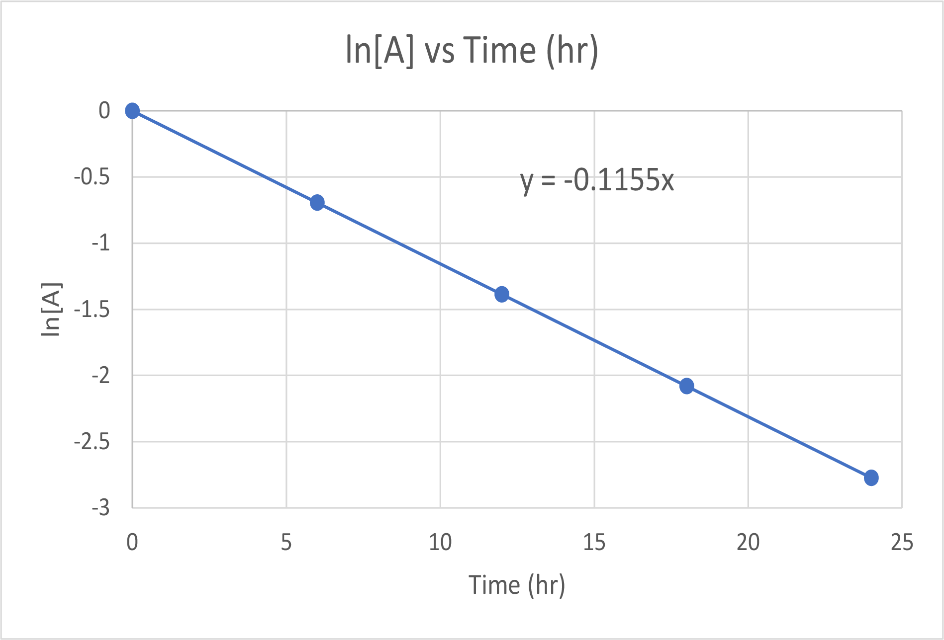
The plot of ln[A] versus time is linear, thus we have verified that the reaction may be described by a first-order rate law.

The rate constant for a first-order reaction is equal to the negative of the slope of the plot of ln[H₂O₂] versus time where:

slope = $\dfrac{\Delta\;y}{\Delta\;x} = \dfrac{\Delta\;\ln[\text{A}]}{\Delta\;t}$

slope = $\dfrac{-1.386\;-\;(-0.693)}{12.00 \text{h}\;-\;6.00 \text{h}}$ = -0.1155 hr^-1

Check Your Learning
Graph the following data to determine whether the reaction, A → B + C, is first order.

Trial	Time (s)	[A] (M)
1	4.0	0.220
2	8.0	0.144
3	12.0	0.110
4	16.0	0.088
5	20.0	0.074

Answer:

The plot of ln[A] vs. t is not a straight line. The equation is not first order.

Second-Order Reactions

For the second-order reaction:

A → Product

the rate is:

rate = $\dfrac{-\Delta[\text{A}]}{\Delta\;t}$

Because this is a second-order reaction, the rate law is:

rate = k[A]²

These two expressions can be combined:

rate = $\dfrac{-\Delta[\text{A}]}{\Delta\;t}$ = k[A]²

Calculus can used to integrate this expression to give us a useful equation relating the rate constant, k, with [A]₀, the initial concentration, and [A]_t, the concentration after time, t, has passed.

$\dfrac{1}{[\text{A}]_{t}}$ = kt + $\dfrac{1}{[\text{A}]_{0}}$

Example 3

The Integrated Rate Law for a Second-Order Reaction
The reaction of butadiene gas (C₄H₆) with itself produces C₈H₁₂ gas as follows:

2 C₄H₆(g) → C₈H₁₂(g)

The reaction is second order with a rate constant equal to 5.76 × 10⁻²M^-1min^-1 under certain conditions. If the initial concentration of butadiene is 0.200 M, what is the concentration remaining after 10.0 min?

Solution
We use the integrated form of the rate law to answer questions regarding time. For a second-order reaction, we have:

We know three variables in this equation: [A]₀ = 0.200 M, k = 5.76 × 10⁻² M^-1min^-1, and t = 10.0 min. Therefore, we can solve for [A], the fourth variable:

$\dfrac{1}{[\text{A}]_{t}}$ = (5.76 x 10^-2 M^-1min^-1) × (10.0 min) + $\dfrac{1}{0.200 \text{M}}$

$\dfrac{1}{[\text{A}]_{t}}$ = 5.58 M^-1

[A] = 0.179 M

Therefore 0.179 M of butadiene remain at the end of 10.0 min, compared to the 0.200 M that was originally present.

Check Your Learning
If the initial concentration of butadiene is 0.0200 M, what is the concentration remaining after 20.0 min?

Answer:

0.0195 M

As with a first-order reaction, we can use integrated rate laws with experimental data of concentration and time over the course of a reaction to graphically determine the order and rate constant of a reaction.

The integrated rate law can be rearranged to a standard linear equation format (y = mx + b, where m = slope and b = the y-intercept):

$\dfrac{1}{[\text{A}]_{t}}$	=	kt	+	$\dfrac{1}{[\text{A}]_{0}}$
y	=	mx	+	b

Thus, a plot of $\frac{1}{[\text{A}]}$ versus t for a second-order reaction is a straight line with a slope of +k and a y-intercept of $\frac{1}{[\text{A}]_{0}}$ . If a set of rate data are plotted in this fashion but do not result in a straight line, the reaction is not second order in A.

A graph is shown with the label “Time” on the x-axis and “[A]” on the y-axis. It has a curved line A second graph is shown with the label “Time” on the x-axis and “1/[A]” on the y-axis. This graph has a positively sloped linear line with a non-zero y-intercept. — **Figure 2:** The linear relationship between the 1/[A] and time shows that the decomposition of A is a second-order reaction.

Example 4

Determination of Reaction Order by Graphing

Test the data given to show whether the dimerization of C₄H₆ is a first- or a second-order reaction.

Solution

Time (s)	[C₄H₆] (M)
0	1.00 × 10⁻²
1600	5.04 × 10⁻³
3200	3.37 × 10⁻³
4800	2.53 × 10⁻³
6200	2.08 × 10⁻³

In order to distinguish a first-order reaction from a second-order reaction, we plot ln[C₄H₆] versus t and compare it with a plot of $\frac{1}{[\text{C}_{4}\text{H}_{6}]}$ versus t. The data used for these plots in in the table below:

Time (s)	$\bfseries{\frac{1}{[\text{C}_{4}\text{H}_{6}]}}$ (M^-1)	ln[C₄H₆]
0	100	−4.605
1600	198	−5.289
3200	296	−5.692
4800	395	−5.978
6200	481	−6.175

The plots are shown below. As you can see, the plot of ln[C₄H₆] versus t is not linear, therefore the reaction is not first order. The plot of $\frac{1}{[\text{C}_{4}\text{H}_{6}]}$ versus t is linear, indicating that the reaction is second order.

Two graphs are shown, each with the label “Time ( s )” on the x-axis. The graph on the left is labeled, “l n [ C subscript 4 H subscript 6 ],” on the y-axis. The graph on the right is labeled “1 divided by [ C subscript 4 H subscript 6 ],” on the y-axis. The x-axes for both graphs show markings at 3000 and 6000. The y-axis for the graph on the left shows markings at negative 6, negative 5, and negative 4. A decreasing slightly concave up curve is drawn through five points at coordinates that are (0, negative 4.605), (1600, negative 5.289), (3200, negative 5.692), (4800, negative 5.978), and (6200, negative 6.175). The y-axis for the graph on the right shows markings at 100, 300, and 500. An approximately linear increasing curve is drawn through five points at coordinates that are (0, 100), (1600, 198), (3200, 296), and (4800, 395), and (6200, 481). — These three graphs show zero-, first- and second-order plots for the dimerization of C₄H₆. Since the zero-order and first-order plots (left, middle) are not linear, we know that the reaction is not zero nor first order. The linear trend in the second-order plot (right) indicates that the reaction follows second-order kinetics.

Check Your Learning: Does the following data fit a second-order rate law?

Time (s)	[A] (M)
5	0.952
10	0.625
15	0.465
20	0.370
25	0.308
35	0.230

Answer:

Yes. The plot of $\frac{1}{[\text{A}]}$ vs. t is linear.

Zero-Order Reactions

For the zero-order reaction:

A → Product

the rate is:

rate = $\dfrac{-\Delta[\text{A}]}{\Delta\;t}$

Because this is a zero-order reaction, the rate law is:

rate = k[A]⁰ = k

These two expressions can be combined:

rate = $\dfrac{-\Delta[\text{A}]}{\Delta\;t}$ = k

Calculus can used to integrate this expression to give us a useful equation relating the rate constant, k, with [A]₀, the initial concentration, and [A]_t, the concentration after time, t, has passed.

[A]_t	=	-kt	+	[A]₀
y	=	mx	+	b

The integrated rate law for a zero-order reaction has the form of the equation of a straight line. A plot of [A] versus t for a zero-order reaction is a straight line with a slope of −k and a y-intercept of [A]₀.

A graph is shown with the label “Time” on the x-axis and “[A]” on the y-axis. It has a negatively sloped linear line.line — **Figure 3:** The linear relationship between the [A] and time shows that the decomposition of A is a zero-order reaction.

Experimental Technique Using Integrated Rate Laws and the Flooding Method

The integrated rate laws are quite useful when determining the reaction order and rate constants using all the data from a single experimental trial run. However, we’ve only considered integrated rate laws for reactions involving one reactant, whereas many reactions involve two or more reactants—how can we use integrated rate laws to find the reaction order and rate constants for those reactions? From the previous chapter, we can use the “flooding” method, where one reactant is at a much larger concentration than the other, making that reactant appear to have a constant concentration with respect to the concentration change that occurs with the smaller concentration reactant.

Let’s consider the reaction:

A + B → Products

where

rate = k[A]^m[B]ⁿ

To isolate the effect of reactant A on the reaction rate, we can run the reaction under a large excess of reactant B, i.e., flooding the reaction mixture with B so that A is the limiting reagent, and reactant B concentration effectively remains constant during the reaction because its consumption is so small that the change in concentration becomes negligible. Under this condition, the effectively constant B concentration and the k constant can be consolidated into a new a rate constant, k_obs, where:

k_obs = k[B]ⁿ

By replacing k[B]ⁿ with k_obs in the rate law, the rate law can be written as:

rate = k_obs[A]^m

This rate law equation derived from the flooding technique allows us to use the integrated rate laws and experimental data to determine the reaction order with respect to reactant A and k_obs.

After measuring the concentration of A as the reaction progresses, we can produce plots of [A] vs time, ln[A] vs time, and $\frac{1}{[\text{A}]}$ vs time. By identifying which plot results in a linear line of data points, the order of the reaction with respect to A can be determined. The absolute value of the slope of that linear plot will be equal to k_obs. An outline of the strategy to be employed can be seen below.

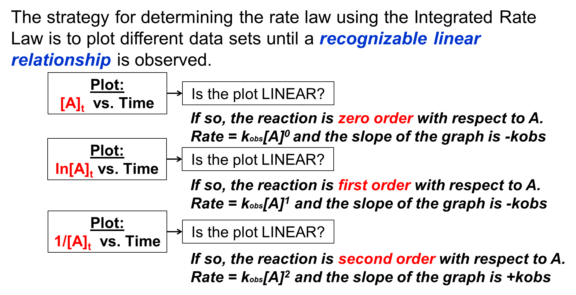
Strategy for assessing the order of reaction with respect to the non-flooded reactant in a flooding experiment.

In this example, after measuring the concentration of A as the reaction progresses, plots of [A] vs time, ln[A] vs time, and $\frac{1}{[\text{A}]}$ vs time are produced, as seen in Figure 4. The ln[A] vs time plot is linear, so the reaction is first-order with respect to A and the slope of the plot equals –k_obs₁ (this experiment will involve a number of trials and so the k_obs has been given a subscript of “1” to keep track of the data).

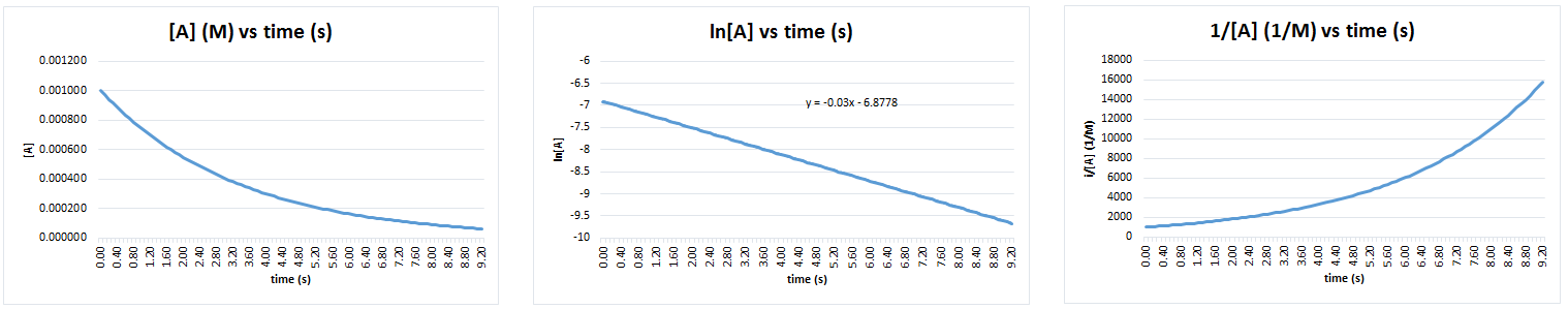
**Figure 4:** Three graphs showing: 1) [A] (M) vs time (s), 2) ln[A] vs time (s), and 3) 1/[A] (1/M) vs time (s). graphs 1 and 3 have curved lines while graph 2 (ln[A] vs time) has a linear curve fit. Each experiment has been performed with a starting concentration of [A] = 0.0010 M and a starting concentration of [B] = 0.1 M.

We can then run another trial with a different concentration of B, 0.2 M, which is still in large excess. The plot of ln[A]_t vs time would will still be linear but will yield a different slope corresponding to -k_obs₂. This can be seen in Figure 5.

**Figure 5:** A graph of ln[A] vs time (s), while varying the concentration of [B].

The ratio of the two k_obs can be used to find the order of B:

$\dfrac{k_{\text{obs}_2}}{k_{\text{obs}_1}} = \dfrac{k[\text{B}]_{2}^n}{k[\text{B}]_{1}^n} = \left(\dfrac{[\text{B}]_2^n}{[\text{B}]_1^n}\right)^{n}$

$\dfrac{0.12}{0.03} = \left(\dfrac{0.2 \text{M}}{0.1 \text{M}}\right)^{n}$

4 = 2ⁿ
n = 2

These values can be put together to find the complete rate law:

rate = k[A][B]²

Key Concepts and Summary

By integrating the first, second, and zero order rate laws, an equation that relates the rate constant, the time (t), the initial concentration of a reactant, and the concentration of the reactant at time, t. These integrated rate laws are powerful tools that, after we know the order of the reactant, we can predict how long it will take for a reaction to occur or how much reactant will be remaining after a certain amount of time. The slope of an integrated rate law plot can be used to find the rate constant, k. We can also use our understanding of flooding from the previous section and relate it to integrated rate laws to find the order of each reactant in a simple way. Most commonly, the plot axes of a linear plot give us the order of the reactant on the graph y-axis. Then, the initial slopes can be compared to find the order of the flooded reactant.

Key Equations

First Order: ln [A]_t = –kt + ln [A]₀ or [A]_t = [A]₀e^–kt
Second Order: $\dfrac{1}{[\text{A}]_{t}}$ = kt + $\dfrac{1}{[\text{A}]_{0}}$
Zero Order: [A]_t = –kt + [A]₀
Flooding: rate = k[A]^m[B]ⁿ | rate = k_obs[A]^m | k_obs = k[B]ⁿ

Glossary

integrated rate laws: a form of each rate law that relates the concentration of reactants and time

Chemistry End of Section Exercises

Describe how graphical methods can be used to determine the order of a reaction and its rate constant from a series of data that includes the concentration of A at varying times.
The reaction: 2 NO₂(g) → 2 NO(g) + O₂(g) is suspected to be second-order. Which of the following kinetic plots would be the most useful to confirm whether or not the reaction is second-order?
1. A plot of 1/[NO₂] vs. t
2. A plot of ln[NO₂] vs. t
3. A plot of [NO₂] vs. t
4. A plot of ln(1/[NO₂]) vs. t
5. A plot of [NO₂]² vs. t
Use the data provided to graphically determine the order and rate constant of the following reaction:
SO₂Cl₂(g) → SO₂(g) + Cl₂(g)

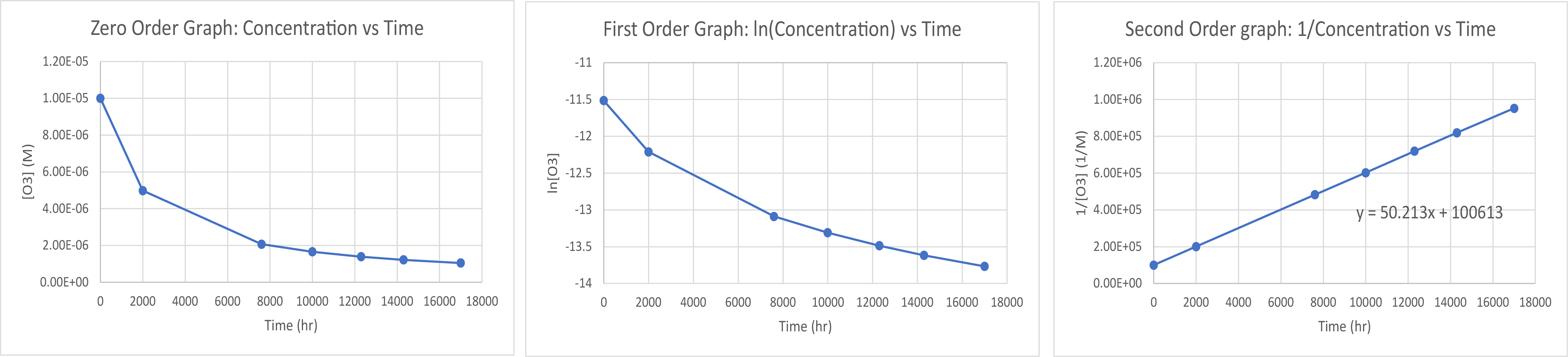
Time (s) [SO₂Cl₂] (M)

0 0.100

5.00 × 10³ 0.0896

1.00 × 10⁴ 0.0802

1.50 × 10⁴ 0.0719

2.50 × 10⁴ 0.0577

3.00 × 10⁴ 0.0517

4.00 × 10⁴ 0.0415
Pure ozone decomposes slowly to oxygen, 2 O₃(g) → 3 O₂(g). Use the data provided in a graphical method and determine the order and rate constant of the reaction.

Time (h) [O₃] (M)

0 1.00 × 10^-5

2.0 × 10³ 4.98 × 10^-6

7.6 × 10³ 2.07 × 10^-6

1.00 × 10⁴ 1.66 × 10^-6

1.23 × 10⁴ 1.39 × 10^-6

1.43 × 10⁴ 1.22 × 10^-6

1.70 × 10⁴ 1.05 × 10^-6
You are asked to calculate a how much of a reactant is left after a certain period of time for a spontaneous zero-order decomposition reaction; however, you have been given three possible rate constants: 0.100 M^-1 s^-1, 0.0075 M s^-1, and 7.5 x 10³ s^-1. Which rate constant should you use and why did you choose that one?
The thermal decomposition of phosphine gas, PH₃, into elemental phosphorous, P₄ (a gas), and hydrogen gas is a first-order reaction, with k = 0.0198 s^-1 at room temperature.
1. Write the balanced reaction for this process.
2. If 0.125 g of PH₃ is allowed to decompose, how much is left after 2.50 minutes?
3. How long will it take for 65% of a phosphine sample to decompose?
The rate constant for the reaction:
2 NOBr(g) → 2 NO(g) + Br₂(g)

is 0.80 M^-1s^-1at 10.0 °C. If the reaction starts with 0.075 M NOBr, what is the concentration of NOBr after 45 seconds?
Determine the rate constant of a zero-order reaction if it takes 3.00 minutes for its initial concentration of 2.00 M to reduce to 0.50 M.
A reaction was experimentally determined to follow the rate law: rate = k[A]², where k = 0.456 M^-1s^-1. If [A]₀ = 0.500 M, how many seconds will it take until [A]_t = 0.250 M?
The reaction of a FDC Blue (a dye use used in food coloring) and hydrogen peroxide, H₂O₂, can be described by the following chemical equation:
FDC Blue(aq) + H₂O₂(aq) → Colorless Products

Although the colorless products have not been characterized, it is known that the two reagents react in a 1:1 stoichiometric ratio.
FDC Blue, as the name suggests, is blue in color, and H₂O₂ is colorless, so that the progress of the reaction can be monitored by following the Absorbance of a reaction mixture in a cuvette with a 1.00 cm pathlength. The molar absorbtivity, ε, of FDC Blue is 8.0 × 10⁵ M^-1cm^-1 at the wavelength used for the measurements. [Recall that Beer’s law relates absorbance (A) to concentration (c), A = εcl, where l is the pathlength.]
The following data is obtained for a reaction where [H₂O₂]₀ = 0.10 M, leading to the three graphs below: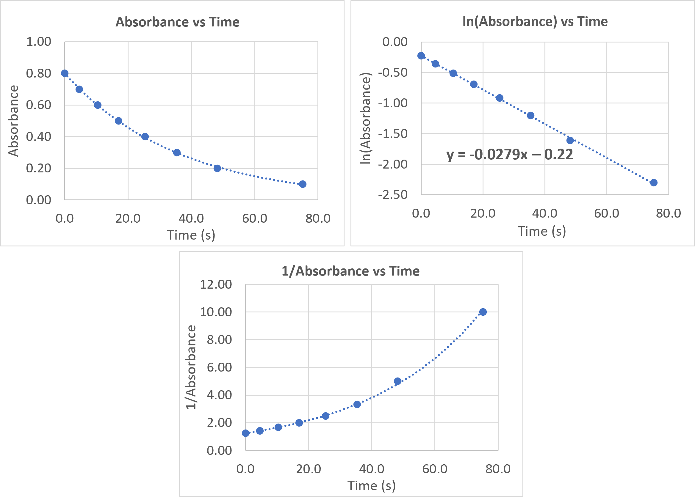
1. What is the initial concentration of the FDC Blue?
2. How has this experiment been designed so that effectively only the concentration of the FDC Blue changes during the course of the reaction?
3. What is the order of the reaction with respect to the [FDC Blue]? Explain your reasoning.
4. A second experiment is undertaken with the [H₂O₂]₀ = 0.050 M, leading to the graphs below:
  
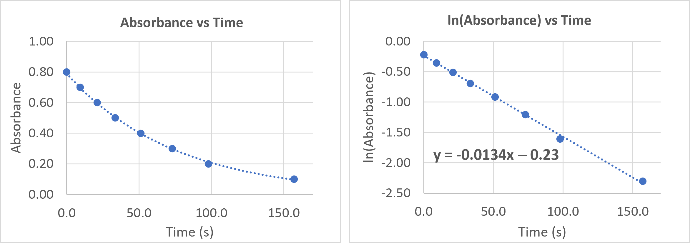
  What is the order of the reaction with respect to [H₂O₂]? Clearly explain/show how you determined your answer.
5. What is the rate law for the reaction?
6. What is the value of the rate constant, k, for the reaction? Include appropriate units.

Answers to Chemistry End of Section Exercises

Using time and concentration data acquired as a reaction progresses may be used to find the order of reactants and the rate constant of a reaction.
- A linear trend line when plotting concentration vs time indicates the order is zero with regard to the reactant. The rate constant is the absolute value of the slope of the trend line.
- A linear trend line when plotting the natural log of concentration vs time indicates the order is first with regard to the reactant. The rate constant is the absolute value of the slope of the trend line.
- A linear trend line when plotting 1/concentration vs time indicates the order is second with regard to the reactant. The rate constant is the absolute value of the slope of the trend line.
This is most simply done when there is only one reactant but may be combined with flooding methods to find orders of reactants when there is more than one reactant present.
A
Plotting a graph of ln[SO₂Cl₂] versus t reveals a linear trend; therefore we know this is a first-order reaction. The best fit slope of the trend line is −2.20 × 10⁵ s⁻¹ so k = 2.20 × 10⁵ s^-1.
Plotting a graph of 1/[O₃] vs time produces a linear trend line, so the reaction is second order. The best fit slope of the trend line is 50.1 M^-1hr^-1 so k = 50.1 M⁻¹ hr⁻¹
0.0075 M s^-1; The rate constant units enable us to determine which is the rate constant.
(a) 4 PH₃(g) → P₄(g) + 6 H₂(g)
(b) 0.00641 g
(c) 53 seconds
0.020 M
0.50 M min^-1
4.39 s
(a) 1.0×10^-6 M
(b) The initial concentration of H₂O₂ is very high compared to the initial concentration of FDC Blue. The reaction has been flooded in H₂O₂, and [H₂O₂] does not change throughout the reaction.
(c) The concentration of FDC Blue is directly proportional to absorbance. A plot of ln(Absorbance) versus time gives a straight line, which indicates the reaction is first order with respect to [FDC Blue].
(d) k_obs = k[H₂O₂]^a. In the first experiment, k_obs = 0.0279 = k[0.10 M]^a; in the second experiment, k_obs = 0.0134 = k[0.050 M]^a. Doubling the concentration of H₂O₂ doubles k_obs, so a= 1 and the reaction is first order with respect to [H₂O₂].
(e) Rate = k[H₂O₂][FDC Blue]
(f) From the first experiment, k = 0.28 M^-1s^-1; from the second experiment, k = 0.27 M^-1s^-1

Comments
Please use this form to report any inconsistencies, errors, or other things you would like to change about this page. We appreciate your comments. 🙂

License

Icon for the Creative Commons Attribution-NonCommercial-ShareAlike 4.0 International License

Chem 103/104 Resource Book Copyright © by Chem 103 Textbook Team and Chem 104 Textbook Team is licensed under a Creative Commons Attribution-NonCommercial-ShareAlike 4.0 International License, except where otherwise noted.

Time (s)	[SO₂Cl₂] (M)
0	0.100
5.00 × 10³	0.0896
1.00 × 10⁴	0.0802
1.50 × 10⁴	0.0719
2.50 × 10⁴	0.0577
3.00 × 10⁴	0.0517
4.00 × 10⁴	0.0415

Time (h)	[O₃] (M)
0	1.00 × 10^-5
2.0 × 10³	4.98 × 10^-6
7.6 × 10³	2.07 × 10^-6
1.00 × 10⁴	1.66 × 10^-6
1.23 × 10⁴	1.39 × 10^-6
1.43 × 10⁴	1.22 × 10^-6
1.70 × 10⁴	1.05 × 10^-6