
M12Q1: Refresher of VSEPR, VBT, and Polarity in Organic Molecules
Learning Objectives
- Identify the molecular geometry of a given atom and the bond angles in organic compounds.
| VSEPR Theory | Molecular Polarity | - Identify hybrid orbitals used in bonding and use hybridization of carbon atoms (sp3, sp2, and sp) to rationalize molecular structure.
| Valence Bond Theory | Hybridization | sp3 | sp2 | sp | - Use strength of intermolecular forces in organic molecules to explain differences in physical properties such as boiling point and solubility.
| Intermolecular Forces |
VSEPR Theory
Valence shell electron-pair repulsion theory (VSEPR theory) enables us to predict the molecular geometry, including approximate bond angles around a central atom, of a molecule from an examination of the number of bonds and lone electron pairs in its Lewis structure. The VSEPR model assumes that electron pairs in the valence shell of a central atom will adopt an arrangement that minimizes repulsions between these electron pairs by maximizing the distance between them. The electrons in the valence shell of a central atom form either bonding pairs or nonbonding lone pairs. The electrostatic repulsion of these electrons is reduced when they assume positions as far away from each other as possible.
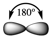
As a simple example of VSEPR theory, let us predict the structure of a gaseous BeF2 molecule. The Lewis structure of BeF2 (Figure 1) shows only two electron pairs around the central beryllium atom. With two bonds and no lone pairs of electrons on the central atom, the bonds are as far apart as possible, and the electrostatic repulsion between these regions of high electron density is reduced to a minimum when they are on opposite sides of the central atom. The F-Be-F bond angle is 180° (Figure 1) in the BeF2 molecule resulting in a linear geometry.

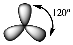
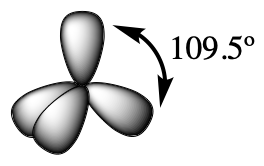
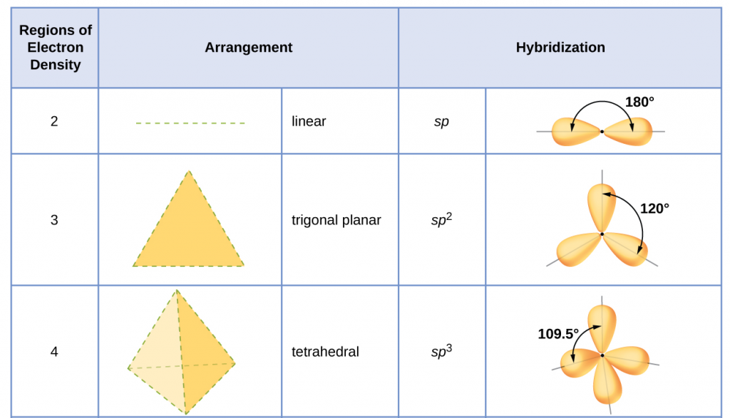
Table 1 illustrates electron region geometries that minimize the repulsions between regions of high electron density (bonds and/or lone pairs). Two regions of electron density around a central atom in a molecule form a linear geometry; three regions form a trigonal (or triangular) planar geometry; and four regions form a tetrahedral geometry.


Electron Region Geometry versus Molecular Geometry
It is important to note that electron region geometry around a central atom is not the same thing as its molecular geometry. The electron region geometries shown in Table 1 describe all regions where electrons are located. Bonds and lone pairs are treated equally. Molecular geometry describes the location of the atoms, not the lone pairs of electrons. The electron region geometries will be the same as the molecular geometries when there are no lone pairs of electrons around the central atom, but they will be different when there are lone pairs present on the central atom.
For example, the methane molecule, CH4, which is the major component of natural gas, has four bonding pairs of electrons around the central carbon atom; the electron region geometry is tetrahedral, as is the molecular geometry (Figure 2). On the other hand, the ammonia molecule, NH3, also has four electron pairs associated with the nitrogen atom, and thus has a tetrahedral electron region geometry. However, one of these regions is a lone pair and this lone pair influences the shape of the molecule, giving it a molecular geometry of trigonal pyramidal (Figure 3).

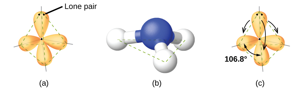
As seen in Figure 3, small distortions from the ideal angles in Table 1 can result from differences in repulsion between various regions of electron density. VSEPR theory predicts these distortions by establishing an order of repulsions and an order of the amount of space occupied by different kinds of electron pairs. This order of repulsions determines the amount of space occupied by different regions of electrons. A lone pair of electrons occupies a larger region of space than the electrons in a triple bond; in turn, electrons in a triple bond occupy more space than those in a double bond, and so on. The order of sizes from largest to smallest is:
lone pair > triple bond > double bond > single bond
Consider formaldehyde, H2CO, which is used as a preservative for biological and anatomical specimens (seen below). This molecule has regions of high electron density that consist of two single bonds and one double bond. The basic geometry is trigonal planar with 120° bond angles, but we see that the double bond causes slightly larger angles (121°), and the angle between the single bonds is slightly smaller (118°).

In the ammonia molecule, the three hydrogen atoms attached to the central nitrogen are not arranged in a flat, trigonal planar molecular geometry, but rather in a three-dimensional trigonal pyramid (Figure 3) with the nitrogen atom at the apex and the three hydrogen atoms forming the base. The ideal bond angles in a trigonal pyramidal structure are based on the tetrahedral electron pair geometry. Again, there are slight deviations from the ideal because lone pairs occupy larger regions of space than do bonding electrons. The H–N–H bond angles in NH3 are slightly smaller than the 109.5° angle in a regular tetrahedron (Table 1) because the lone pair of electrons occupy more space than a single bond (Figure 3). Table 2 illustrates the ideal molecular geometry predicted for a given combination of lone pairs and bonding pairs.
Predicting Electron Pair Geometry and Molecular Geometry
The following procedure uses VSEPR theory to determine the electron pair geometry and molecular geometry for a given molecule:
- Draw the Lewis structure of the molecule or polyatomic ion.
- Count the number of regions of electron density (lone pairs and bonds) around the central atom. A single, double, or triple bond counts as one region of electron density.
- Identify the electron region geometry based on the number of regions of electron density: linear, trigonal planar, or tetrahedral (Table 2, first column).
- Use the number of lone pairs to determine the molecular geometry (Table 2).
Molecular Geometry for Multicenter Molecules
When a molecule or polyatomic ion only has one central atom, the molecular geometry completely describes the shape of the molecule. Larger molecules do not have a single central atom, but are connected by a chain of interior, central atoms that each possess a “local” geometry. The way these local structures are oriented with respect to each other also influences the molecular shape, but such considerations are largely beyond the scope of this introductory discussion. For our purposes, we will only focus on determining the local geometries of single atoms.
Example 1
Predicting Geometries in Multicenter Molecules
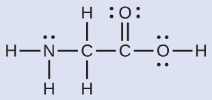
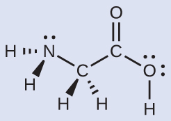
The Lewis structure for the simplest amino acid, glycine, H2NCH2CO2H, is shown here. Predict the electron region geometry and local molecular geometry for the nitrogen atom and the two carbon atoms:
Solution
Consider each central atom independently. The electron region geometries:
- nitrogen––four regions of electron density; tetrahedral
- carbon (CH2)––four regions of electron density; tetrahedral
- carbon (CO2)—three regions of electron density; trigonal planar
The local molecular geometry:
- nitrogen––three bonds, one lone pair; trigonal pyramidal
- carbon (CH2)—four bonds, no lone pairs; tetrahedral
- carbon (CO2)—three bonds (double bond counts as one bond), no lone pairs; trigonal planar
Check Your Learning
Another amino acid is alanine, which has the Lewis structure shown here. Predict the electron region geometry and local molecular geometry of the nitrogen atom and the three carbon atoms:
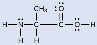
Answer:
electron region geometries: nitrogen––tetrahedral; carbon (CH)—tetrahedral; carbon (CH3)—tetrahedral; carbon (CO2)—trigonal planar
local molecular geometry: nitrogen—trigonal pyramidal; carbon (CH)—tetrahedral; carbon (CH3)—tetrahedral; carbon (CO2)—trigonal planar
Molecular Polarity and Dipole Moment
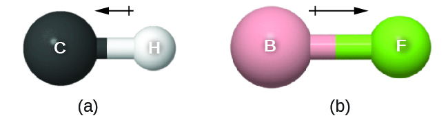
As discussed previously, polar covalent bonds connect two atoms with differing electronegativities, leaving one atom with a partial positive charge (δ+) and the other atom with a partial negative charge (δ–), as the electrons are pulled toward the more electronegative atom. This separation of charge gives rise to a bond dipole moment. This bond dipole moment can be represented as a vector, a quantity having both direction and magnitude (Figure 4). Dipole vectors are shown as arrows pointing along the bond from the less electronegative atom toward the more electronegative atom. A small plus sign is drawn on the less electronegative end to indicate the partially positive end of the bond. The length of the arrow is proportional to the magnitude of the electronegativity difference between the two atoms. For this class, you should memorize these trends of electronegativity: F > O > N > Cl >> … > C > … > H > metals
A whole molecule may also have a dipole moment, depending on its molecular geometry and the polarity of each of its bonds. If the molecule does have a dipole moment, the molecule is said to be a polar molecule; otherwise the molecule is said to be nonpolar. The molecular dipole moment measures the net charge separation in the whole molecule. We determine the molecular dipole moment by adding all of the bond dipole moments in three-dimensional space.
Homonuclear diatomic molecules, such as Br2 and N2, have bond and molecular dipole moments equal to zero, because the two component atoms have equal electronegativity. For heteronuclear molecules, such as CO or HF, the molecular dipole moment is equal to the bond dipole moment, which is determined by the magnitude of difference between the two electronegativity values.
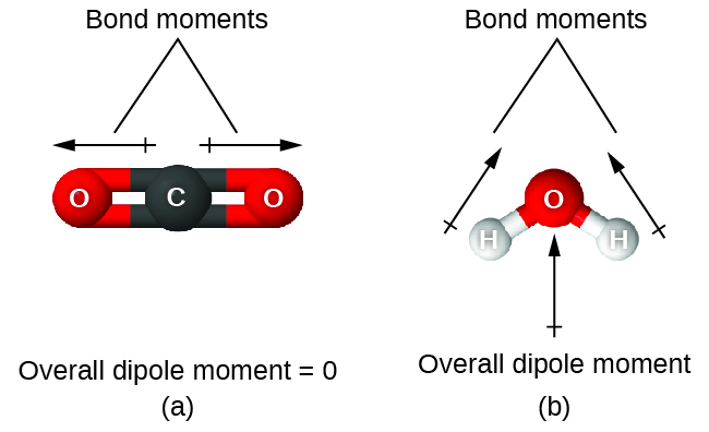
When a molecule contains more than one bond, the geometry must be taken into account. If the bonds in a molecule are arranged such that their bond dipole moments cancel (vector sum equals zero), then the molecule is nonpolar. This is the situation in CO2 (Figure 5). Each of the C=O bonds are polar, but the molecule as a whole is nonpolar. From the Lewis structure and using VSEPR theory, we determine that the CO2 molecule is linear with polar C=O bonds on opposite sides of the carbon atom. The bond dipole moments cancel because they are pointed in opposite directions. In the case of the water molecule (Figure 5), the Lewis structure shows that there are two bonds to a central atom, and the electronegativity difference between oxygen and hydrogen indicates that each of these O-H bonds has a nonzero bond dipole moment. In this case, however, the molecular geometry is bent because of the lone pairs on oxygen, and the two bond dipole moments do not cancel out. Therefore, water does have a net molecular dipole moment and is therefore a polar molecule.
The OCS molecule has a structure similar to CO2, but a sulfur atom has replaced one of the oxygen atoms. To determine if this molecule is polar, we first draw the molecule with the correct geometry. VSEPR theory predicts a linear molecule:
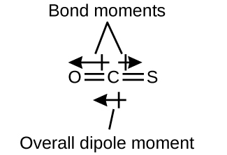
The C-O bond is considerably polar. Although C and S have very similar electronegativity values, S is slightly more electronegative than C, and so the C-S bond is just slightly polar. Even though these bond dipole moments are pointing in opposite directions, they will not fully cancel because they have different magnitudes. Since oxygen is more electronegative than sulfur, the overall molecular dipole moment will point towards the oxygen end of the molecule.
Chloromethane, CH3Cl, is another example of a polar molecule. Although the polar C–Cl and C–H bonds are arranged in a tetrahedral geometry, the C–Cl bond has a larger bond dipole moment than the C–H bonds, and the bond dipole moments do not cancel each other out. All of the dipoles have an upward component in the orientation shown, since carbon is more electronegative than hydrogen and less electronegative than chlorine, giving an overall molecular dipole moment going from the hydrogens through the chlorine:

Note that there is a small electronegativity difference between carbon and hydrogen and a C-H bond is slightly polar; however, the difference is quite small, and C-H bonds are often categorized as nonpolar.
The highly symmetrical molecules BF3 (trigonal planar) and CH4 (tetrahedral), in which all the polar bonds are identical and symmetrical, are nonpolar. The bonds in these molecules are arranged such that their bond dipoles cancel. However, just because a molecule contains identical bonds does not mean that the dipoles will always cancel. Many molecules that have identical bonds and lone pairs on the central atoms have bond dipoles that do not cancel. Examples include H2O, H2S, and NH3. A hydrogen atom is at the positive end and a nitrogen or sulfur atom is at the negative end of the polar bonds in these molecules:

In summary, to be polar, a molecule must:
- Contain at least one polar covalent bond.
- Have a molecular geometry such that the sum of the vectors of each bond dipole moment does not equal zero.
Intermolecular Forces
Intermolecular forces (IMF) are the various forces of attraction that exist between atoms and/or molecules due to electrostatic properties. We will often use values such as boiling or melting points as indicators of the relative strengths of IMFs present within different substances. The stronger the IMF, the higher the melting and boiling points, and the lower the vapor pressure. The IMF from Chem 103 (starting with the strongest) are:
- Ion-Ion: the force between two ions (example: NaCl(s))
- Ion-Dipole: the force between an ion and a polar molecule (example: Na+(aq) and H2O(ℓ))
- Dipole-Dipole: the force between two polar molecules.
- Hydrogen Bonding: certain polar molecules containing F, O, or N also exhibit this strong IMF (example: H2O(ℓ) with itself, H2O(ℓ) and NH3(ℓ))
- Dipole-Induced Dipole: the force between a polar molecular and a non-polar molecule (example: H2O(ℓ) and C6H12O6(aq), table sugar)
- London Dispersion Forces, also known as Induced Dipole-Induced Dipole, van der Waal’s, or just Dispersion: the force between any two molecules that each have at least one electron.
For this course, we will focus on Dispersion, Dipole-Dipole, and Hydrogen Bonding forces.
Dispersion Forces
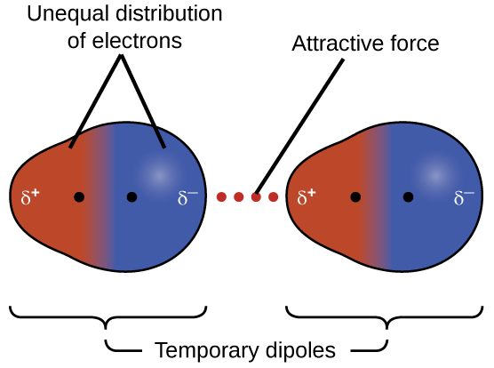
The electrons of an atom or molecule are in constant motion, so at any moment in time, an atom or molecule can develop a temporary, instantaneous dipole if its electrons are distributed asymmetrically. The presence of this dipole can, in turn, distort the electrons of a neighboring atom or molecule, producing an induced dipole. These two rapidly fluctuating, temporary dipoles result in a relatively weak electrostatic attraction between the molecules, a so-called dispersion force, like that illustrated in Figure 6.
Dispersion forces that develop between atoms in different molecules can attract the two molecules to each other. The forces are relatively weak and only become significant when the molecules are very close. Larger and heavier atoms and molecules exhibit stronger dispersion forces than those found in smaller and lighter atoms and molecules. F2 and Cl2 are gases at room temperature (reflecting weaker dispersion forces); Br2 is a liquid, and I2 is a solid (reflecting stronger dispersion forces).
The increase in melting and boiling points with increasing atomic/molecular size may be rationalized by considering how the strength of dispersion forces is affected by the electronic structure of the substance. In a larger atom, the valence electrons are, on average, farther from the nuclei than in a smaller atom. Thus, they are less tightly held and can more easily form the temporary dipoles that produce the attraction. The measure of how easy or difficult it is for another electrostatic charge (for example, a nearby ion or polar molecule) to distort a molecule’s charge distribution (its electron cloud) is known as polarizability. A molecule that has a charge cloud that is easily distorted is said to be very polarizable and will have large dispersion forces; one with a charge cloud that is difficult to distort is not very polarizable and will have small dispersion forces.
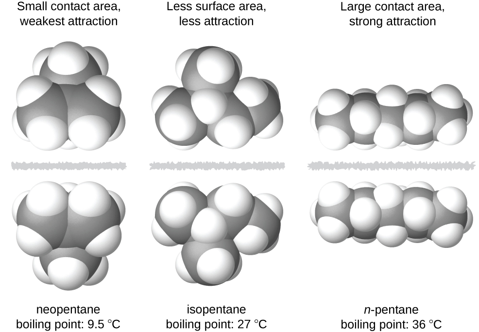
The shapes of molecules also affect the magnitudes of the dispersion forces between them. For example, boiling points for the isomers n-pentane, isopentane, and neopentane (shown in Figure 7) are 36 °C, 27 °C, and 9.5 °C, respectively. Even though these compounds all have the same empirical formula, C5H12, the difference in boiling points suggests that dispersion forces in the liquid phase for each are different, the greatest seen in n-pentane and the weakest in neopentane. The elongated shape of n-pentane provides a greater surface area available for contact between molecules, resulting in correspondingly stronger dispersion forces. The more compact shape of isopentane offers a smaller surface area available for intermolecular contact and, therefore, results in weaker dispersion forces. Neopentane molecules are the most compact of the three, offering the least available surface area for intermolecular contact and, hence, the weakest dispersion forces. This behavior is analogous to the connections that may be formed between strips of VELCRO brand fasteners: the greater the area of the strip’s contact, the stronger the connection.
Dipole-Dipole Forces
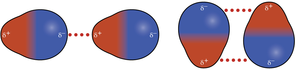
Recall from earlier in this section that polar molecules have a partial positive charge on one side of the molecule and a partial negative charge on the other side—a separation of charge called a dipole. Consider a polar molecule such as hydrogen chloride, HCl. In the HCl molecule, the less electronegative H atom bears the partial positive charge (shown in red in Figure 12) and the more electronegative Cl atom bears the partial negative charge (shown in blue). An attractive force between HCl molecules results from the attraction between the positive end of one HCl molecule and the negative end of another. This attractive force is called a dipole-dipole attraction—the electrostatic force between the partially positive end of one polar molecule and the partially negative end of another, as illustrated in Figure 8.
The effect of a dipole-dipole attraction is apparent when we compare the properties of HCl molecules to nonpolar F2 molecules. Both HCl and F2 consist of the same number of atoms and have approximately the same molecular mass. However, the dipole-dipole attractions between HCl molecules are sufficient to cause them to “stick together” to form a liquid, whereas the relatively weaker dispersion forces between nonpolar F2 molecules are not, and so F2 is gaseous at this temperature. The higher boiling point of HCl (188 K) compared to F2 (85 K) is a reflection of the greater strength of dipole-dipole attractions between HCl molecules, compared to the attractions between nonpolar F2 molecules.
Hydrogen-Bonding Forces
Nitrosyl fluoride (ONF, molecular mass 49 g/mol) is a gas (weak IMF) at room temperature. Water (H2O, molecular mass 18 g/mol) is a liquid (stronger IMF), even though it has a lower molecular mass. We clearly cannot attribute this difference of physical state between the two compounds to dispersion forces. Both molecules have about the same shape and ONF is the heavier and larger molecule. It is, therefore, expected to experience more significant dispersion forces. Additionally, we cannot attribute this difference in boiling points to differences in the dipole moments of the molecules. Both molecules are polar and exhibit comparable dipole moments.

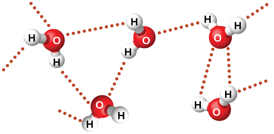
The large difference between the boiling points is due to a particularly strong dipole-dipole attraction that may occur when a molecule contains a hydrogen atom bonded to a fluorine, oxygen, or nitrogen atom (the three most electronegative elements). The very large difference in electronegativity between the H atom and the atom to which it is bonded (F, O, or N), combined with the very small size of a H atom and the relatively small sizes of F, O, or N atoms, leads to highly concentrated partial charges with these atoms. Molecules with F-H, O-H, or N-H bonds are very strongly attracted to lone pairs on F, O, or N in nearby molecules, a particularly strong type of dipole-dipole attraction called hydrogen bonding. Examples of hydrogen bonds include HF⋯HF, H2O⋯HOH, and H3N⋯HNH2, in which the hydrogen bonds are denoted by dots. Figure 9 illustrates hydrogen bonding between water molecules.
Despite use of the word “bond,” keep in mind that hydrogen bonds are intermolecular attractive forces, not intramolecular (covalent bonds). Hydrogen bonds are much weaker than covalent bonds, only about 5 to 10% as strong, but are generally much stronger than other dipole-dipole attractions and dispersion forces.
Demonstration: Immiscibility of Molecules based on Chain Length
Set up. In this demonstration, water with green food coloring is added to four graduated cylinders, each containing a different liquid: ethanol, 1-propanol, 1-butanol, and 1-hexanol.
Prediction.For each liquid, predict whether it will be miscible or immiscible with the added water.
Explanation. In order for two molecules to be miscible, they must have similar intermolecular forces. Water is a polar molecule and is only miscible with other molecules that are also polar. Although each of the four molecules that were mixed with water were alcohols, as the carbon-chain length increases, the majority of the molecule becomes non-polar. This is why ethanol and propanol are miscible with water, but alcohols with any longer carbon-chain are immiscible. This phenomenon is known as “like dissolves like”.
Valence Bond Theory
Valence bond theory describes a covalent bond as the overlap of two half-filled atomic orbitals (each containing a single electron) that yield a pair of electrons shared between the two bonded atoms. We say that orbitals on two different atoms overlap when a portion of one orbital and a portion of a second orbital occupy the same region of space. The strength of a covalent bond depends on the extent of overlap of the orbitals involved. Orbitals that overlap extensively form bonds that are stronger than those that have less overlap.
The energy of a given system depends on how much the orbitals overlap. Figure 10 illustrates how the sum of the energies (the red curve) in a system containing only two hydrogen atoms changes as they approach each other. When the atoms are far apart (to the right on the red curve) there is no overlap, and by convention we set the sum of the energies at zero. As the atoms move together (moving from right to left), their orbitals begin to overlap. Each electron begins to feel the attraction of the nucleus in the other atom. In addition, the electrons begin to repel each other, as do the nuclei. While the atoms are still widely separated, the attractions are slightly stronger than the repulsions, and the energy of the system decreases and a bond begins to form. As the atoms move closer together (to the left on the red curve), the overlap increases, so the attraction of the nuclei for the electrons continues to increase (as do the repulsions among electrons and between the nuclei). At some specific distance between the atoms, which varies depending on the atoms involved, the energy reaches its lowest (most stable) value. This optimum distance between the two bonded nuclei is the bond distance between the two atoms. The bond is stable because at this point, the attractive and repulsive forces combine to create the lowest possible energy configuration. If the distance between the nuclei were to decrease further, the repulsions between nuclei and the repulsions as electrons are confined in closer proximity to each other would become stronger than the attractive forces. The energy of the system would then rise (making the system less stable), as shown at the far left of Figure 10.
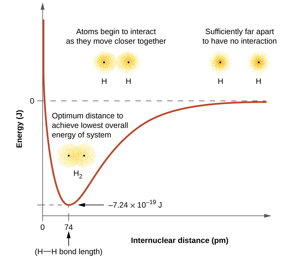
The bond energy is the difference between the energy minimum (which occurs at the bond distance) and the energy of the two separated atoms (which is defined as zero). This is the quantity of energy released when the bond is formed. Conversely, the same amount of energy is required to break the bond. For the H2 molecule shown in Figure 10, at the bond distance of 74 pm the system is 7.24 × 10⁻¹⁹ J lower in energy than the two separated hydrogen atoms. This may seem like a small number. However, we know from our earlier description of thermochemistry that bond energies are often discussed on a per-mole basis. For example, it requires 7.24 × 10⁻¹⁹ J to break one H–H bond, but it takes 4.36 × 10⁵ J to break 1 mole of H–H bonds. A comparison of some bond lengths and energies is shown in Table 3 for your reference. We can find many of these bonds in a variety of molecules, and this table provides average values. For example, breaking the first C–H bond in CH4 requires 439.3 kJ/mol, while breaking the first C–H bond in H–CH2C6H5 (a common paint thinner) requires 375.5 kJ/mol.
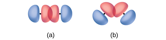
In addition to the distance between two orbitals, the orientation of orbitals also affects their overlap (other than for two s orbitals, which are spherically symmetric). Greater overlap is possible when orbitals are oriented such that they overlap on a direct line between the two nuclei. Figure 11 illustrates this for two p orbitals from different atoms; the overlap is greater when the orbitals overlap end to end (in part a) rather than at an angle (in part b).
The overlap of two s orbitals (as in H2), the overlap of an s orbital and a p orbital (as in HCl), and the end-to-end overlap of two p orbitals (as in Cl2) all produce sigma bonds (σ bonds), as illustrated in Figure 12. A σ bond is a covalent bond in which the electron density is concentrated in the region along the internuclear axis. This is sometimes referred to as a head-to-head interaction. Single bonds in Lewis structures are described as σ bonds in valence bond theory.
A pi bond (π bond) is a type of covalent bond that results from the side-to-side overlap of two p orbitals, as illustrated in Figure 13. In a π bond, the regions of orbital overlap lie on opposite sides of the internuclear axis. Along the axis itself, there is a node, which is a plane with no probability of finding an electron.

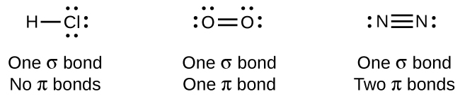
While all single bonds are σ bonds, multiple bonds consist of both σ and π bonds. As the Lewis structures suggest, O2 contains a double bond and N2 contains a triple bond. The double bond consists of one σ bond and one π bond, and the triple bond consists of one σ bond and two π bonds. Between any two atoms, the first bond formed will always be a σ bond, but there can only be one σ bond in any one location. In any multiple bond, there will be one σ bond, and the remaining one or two bonds will be π bonds.
As seen in Table 3, an average carbon-carbon single bond is 347 kJ/mol, while in a carbon-carbon double bond, the π bond increases the bond strength by 267 kJ/mol (from 347 kJ/mol to 614 kJ/mol). Adding an additional π bond causes a further increase of 225 kJ/mol (to 839 kJ/mol). We can see a similar pattern when we compare other σ and π bonds. Thus, each individual π bond is generally weaker than a corresponding σ bond between the same two atoms. In a σ bond, there is a greater degree of orbital overlap than in a π bond.
Example 2
Counting σ and π Bonds
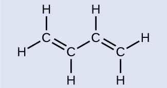
Butadiene, C6H6, is used to make synthetic rubber. Identify the number of σ and π bonds contained in this molecule.
Solution
There are six σ C–H bonds and one σ C–C bond, for a total of seven from the single bonds. There are two double bonds that each have a σ bond and a π bond. This gives a total of nine σ and two π bonds.
Check Your Learning
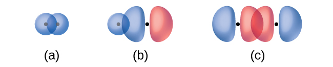
Identify each illustration as depicting a σ or π bond:
- side-by-side overlap of a 4p and a 2p orbital
- end-to-end overlap of a 4p and 4p orbital
- end-to-end overlap of a 4p and a 2p orbital

Answer:
(a) is a π bond that overlaps side-to-side with a node along the axis connecting the nuclei while (b) and (c) are σ bonds that overlap head-to-head along the axis.
Hybrid Orbitals
Thinking in terms of overlapping atomic orbitals is one way for us to explain how covalent bonds form in diatomic molecules. However, to understand how molecules with more than two atoms form stable bonds, we require a more detailed model. As an example, let us consider the water molecule, in which we have one oxygen atom bonding to two hydrogen atoms. Oxygen has the electron configuration 1s22s22p4, with two unpaired electrons (one in each of the two 2p orbitals). Valence bond theory would predict that the two O–H bonds form from the overlap of these two 2p orbitals with the 1s orbitals of the hydrogen atoms. If this were the case, the bond angle would be 90°, as shown in Figure 14[1], because p orbitals are perpendicular to each other. Experimental evidence shows that the bond angle is 104.5°, not 90°. The prediction of the valence bond theory model does not match the real-world observations of a water molecule. A different model is needed.
One widely accepted model that explains observed bond angles in water, and many other molecules, is called hybridization. This model uses quantum mechanics to mathematically combine valence orbitals and create new hybrid orbitals. The details for how this process works is well beyond the scope of this course, but the general principles can be more easily understood.
The following ideas are important in understanding hybridization:
- Hybrid orbitals do not exist in isolated atoms. They are formed only in covalently bonded atoms.
- Hybrid orbitals have shapes and orientations that are very different from those of the atomic orbitals (i.e. s, p, d) in isolated atoms.
- A set of hybrid orbitals is generated by combining atomic orbitals. The number of hybrid orbitals created is equal to the number of atomic orbitals that were combined to produce the hybrid orbitals.
- All orbitals in a set of hybrid orbitals are equivalent in shape and energy.
- The type of hybrid orbitals formed in a bonded atom depends on its electron region geometry as predicted by the VSEPR theory.
- Hybrid orbitals overlap to form σ bonds. Unhybridized orbitals overlap to form π bonds.
In the following sections, we shall discuss the common types of hybrid orbitals.
sp3 Hybridization
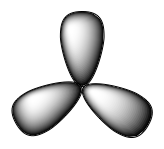
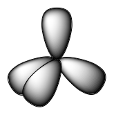
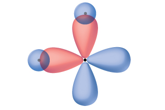
The valence orbitals of an atom surrounded by a tetrahedral arrangement of bonding pairs and lone pairs (like that of H2O or CH4) consist of a set of four sp3 hybrid orbitals. The hybrids result from the mixing of one s orbital and all three p orbitals that produces four identical sp3 hybrid orbitals (Figure 15). Each of these hybrid orbitals points toward a different corner of a tetrahedron.
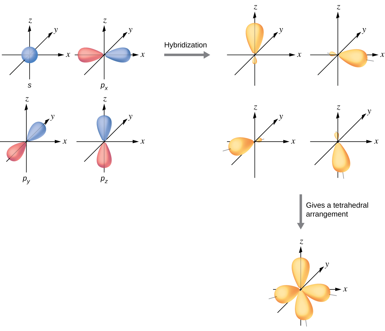
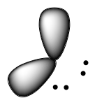
Although quantum mechanics yields the “plump” orbital lobes, sometimes for clarity these orbitals are drawn “thinner” and without the minor lobes, like in the last tetrahedral image in Figure 15, to avoid obscuring other features of a given illustration. We will use these thinner representations whenever the true view is too crowded to easily visualize.
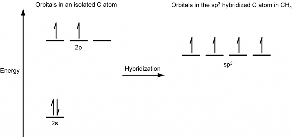
A molecule of methane, CH4, consists of a carbon atom surrounded by four hydrogen atoms at the corners of a tetrahedron. The carbon atom in methane exhibits sp3 hybridization. We illustrate the orbitals and electron distribution in an isolated carbon atom and in the bonded atom in CH4 in Figure 16. The four valence electrons of the carbon atom are distributed equally in the hybrid orbitals, and each carbon electron pairs with a hydrogen electron when the C–H bonds form.
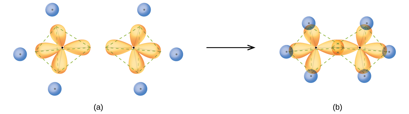
In a methane molecule, the 1s orbital of each hydrogen atoms overlaps with one of the four sp3 orbitals of the carbon atom to form four σ bonds. This results in the formation of four strong, equivalent covalent bonds between the carbon atom and each of the four hydrogen atoms to produce the methane molecule, CH4. The structure of ethane, C2H6, is similar to that of methane in that each carbon in ethane has four neighboring atoms arranged at the corners of a tetrahedron—three hydrogen atoms and one carbon atom (Figure 17).
However, in ethane an sp3 orbital of one carbon atom overlaps end to end with an sp3 orbital of a second carbon atom to form a σ bond between the two carbon atoms. Each of the remaining sp3 hybrid orbitals overlaps with an s orbital of a hydrogen atom to form carbon–hydrogen σ bonds. The structure and overall outline of the bonding orbitals of ethane are shown in Figure 17. The orientation of the two CH3 groups is not fixed relative to each other. Experimental evidence shows that rotation around σ bonds occurs easily.
An sp3 hybrid orbital can also hold a lone pair of electrons. For example, the nitrogen atom in ammonia, NH3, is surrounded by three bonding pairs and a lone pair of electrons directed to the four corners of a tetrahedron. The nitrogen atom is sp3 hybridized with one hybrid orbital occupied by the lone pair.
The molecular structure of water is consistent with a tetrahedral arrangement of two lone pairs and two bonding pairs of electrons. Thus we say that the oxygen atom is sp3 hybridized, with two of the hybrid orbitals occupied by lone pairs and two by bonding pairs. Since lone pairs occupy more space than bonding pairs, structures that contain lone pairs have bond angles slightly distorted from the ideal. Perfect tetrahedra have angles of 109.5°, but the observed angles in ammonia (107.3°) and water (104.5°) are slightly smaller. Other examples of sp3 hybridization include CCl4, PCl3, and NCl3.
sp2 Hybridization
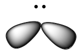
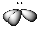
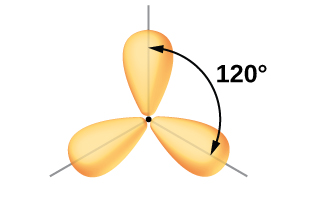
The valence orbitals of a central atom surrounded by three regions of electron density consist of a set of three sp2 hybrid orbitals and one unhybridized p orbital (like that of BH3). This arrangement results from sp2 hybridization, the mixing of one s orbital and two p orbitals to produce three identical hybrid orbitals oriented in a trigonal planar geometry (Figure 18).
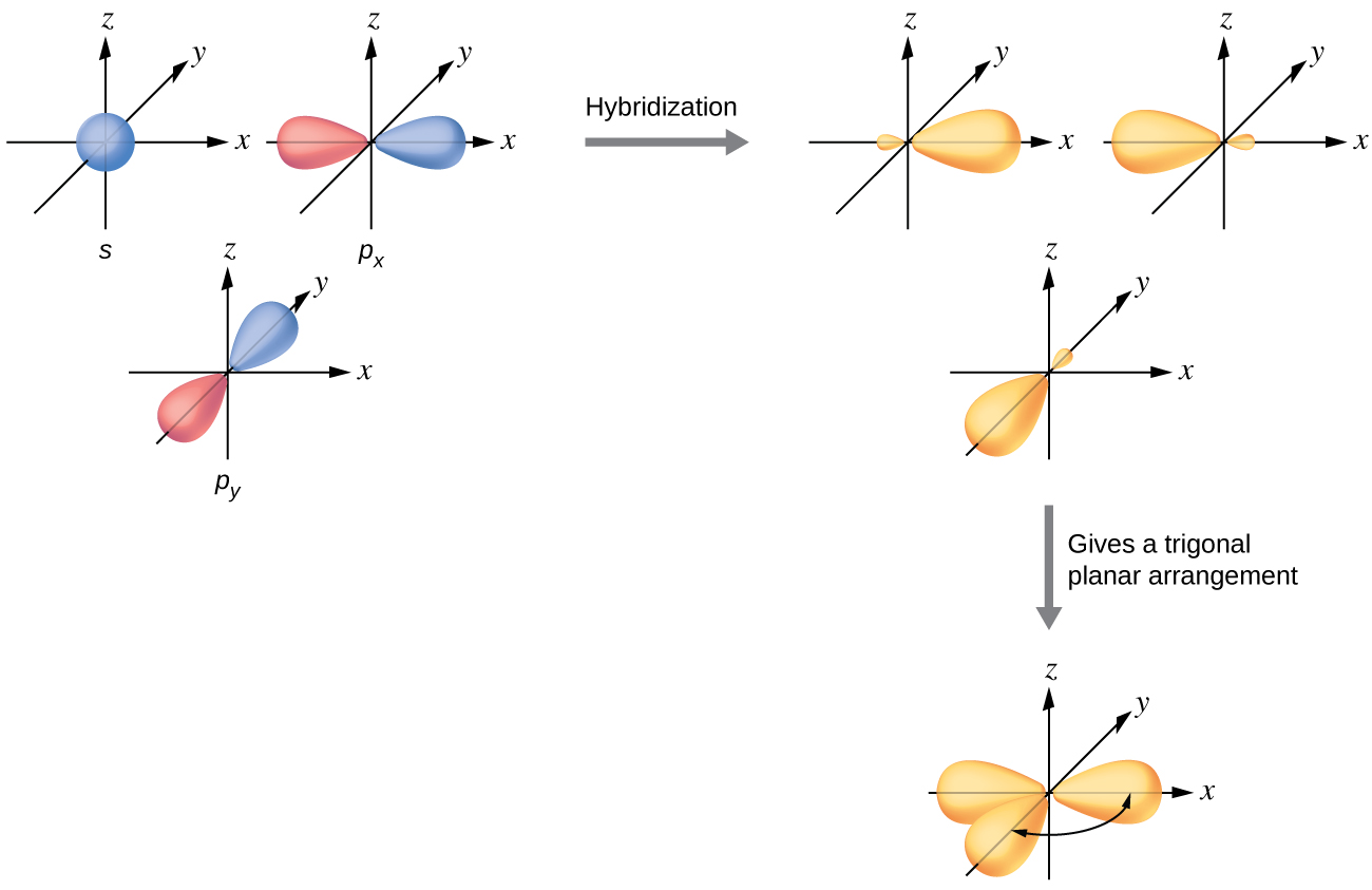
We often use the thinner representation in Figure 19 whenever the true view is too crowded to easily visualize.
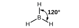
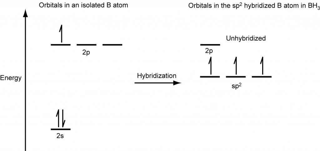
The observed structure of the borane molecule, BH3, suggests sp2 hybridization for boron in this compound. The molecule is trigonal planar, and the boron atom is bonded to three hydrogen atoms (Figure 20). We can illustrate the comparison of orbitals and electron distribution in an isolated boron atom and in the bonded atom in BH3 as shown in the orbital energy level diagram in Figure 21. We redistribute the three valence electrons of the boron atom into the three sp2 hybrid orbitals, and each boron electron pairs with a hydrogen electron when B–H covalent bonds form.
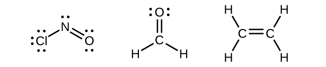
Any central atom surrounded by three regions of electron density will exhibit sp2 hybridization. This includes molecules with a lone pair on the central atom, such as ClNO (Figure 22), or molecules with two single bonds and a double bond connected to the central atom, as in formaldehyde, CH2O, and ethene, H2CCH2.
sp Hybridization
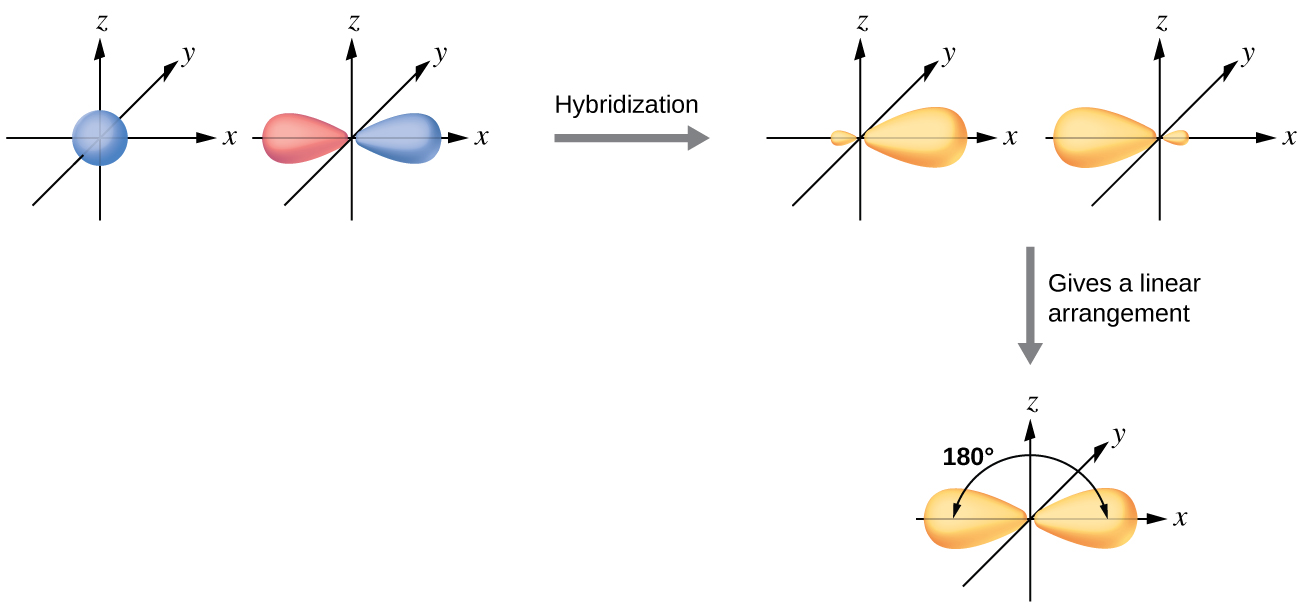
The valence orbitals of an atom surrounded by a linear arrangement of bonding pairs and lone pairs (like that of BeCl2) consist of a set of two sp hybrid orbitals. The hybrids result from the mixing of one s orbital and one p orbitals that produces two identical sp hybrid orbitals (Figure 23). Each of these hybrid orbitals point 180º from each other and the two electrons that were originally in the s orbital are now evenly distributed to the two sp orbitals.
We illustrate the electronic differences in an isolated Be atom and in the bonded Be atom in the orbital energy-level diagram in Figure 24. These diagrams represent each orbital by a horizontal line (indicating its energy) and each electron by an arrow. Energy increases toward the top of the diagram.
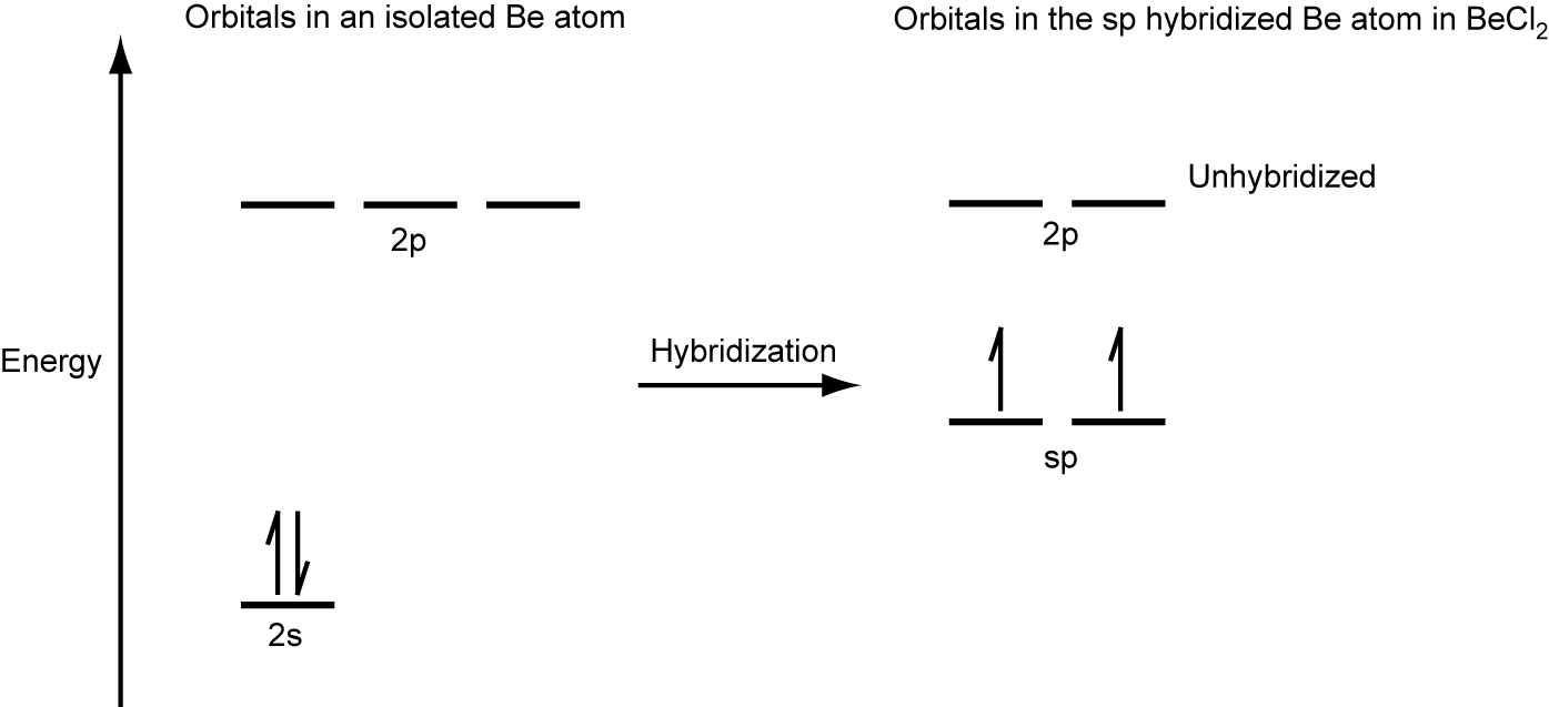
When atomic orbitals hybridize, the valence electrons occupy the newly created orbitals. The Be atom had two valence electrons, so each of the sp orbitals gets one of these electrons. Each of these electrons pairs up with the unpaired electron on a chlorine atom when a hybrid orbital and a chlorine orbital overlap during the formation of the Be–Cl bonds.
Any central atom surrounded by just two regions of valence electron density in a molecule will exhibit sp hybridization. Other examples include the carbon atoms in HCCH and CO2.

Check out the University of Wisconsin-Oshkosh website to learn about visualizing hybrid orbitals in three dimensions.
Assignment of Hybrid Orbitals to Central Atoms
The hybridization of an atom is determined based on the number of regions of electron density that surround it. The geometrical arrangements characteristic of the various sets of hybrid orbitals are shown in Figure 25. These arrangements are identical to those of the electron region geometries predicted by VSEPR theory. VSEPR theory predicts the shapes of molecules, and hybrid orbital theory provides an explanation for how those shapes are formed. To find the hybridization of a central atom, we can use the following guidelines:
- Determine the Lewis structure of the molecule.
- Determine the number of regions of electron density around an atom using VSEPR theory, in which single bonds, multiple bonds, radicals, and lone pairs each count as one region.
- Assign the set of hybridized orbitals from Figure 25 that corresponds to this geometry.
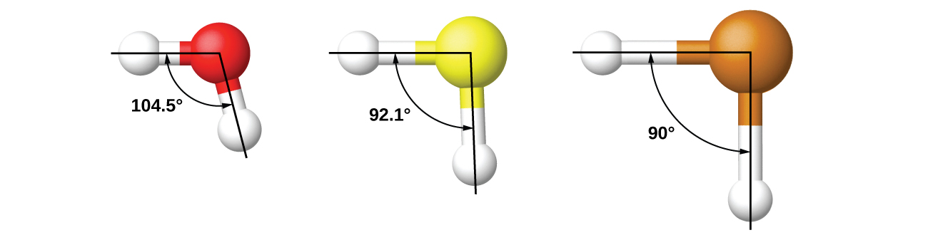
It is important to remember that hybridization was devised to rationalize experimentally observed molecular geometries. The model works well for molecules containing small central atoms, in which the valence electron pairs are close together in space. However, for larger central atoms, the valence-shell electron pairs are farther from the nucleus and there are fewer repulsions. Their compounds exhibit structures that are often not consistent with VSEPR theory and hybridized orbitals are not necessary to explain the observed data. For example, we have discussed the H–O–H bond angle in H2O (in red below), 104.5°, which is more consistent with sp3 hybrid orbitals (109.5°) on the central atom than with 2p orbitals (90°). Sulfur is in the same group as oxygen, and H2S (in yellow) has a similar Lewis structure. However, it has a much smaller bond angle (92.1°), which indicates much less hybridization on sulfur than oxygen. Continuing down the group, tellurium (in brown) is even larger than sulfur, and for H2Te, the observed bond angle (90°) is consistent with overlap of the 5p orbitals, without invoking hybridization. We invoke hybridization where it is necessary to explain the observed structures.
Multiple Bond Hybridization
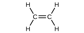
The hybrid orbital model appears to account well for the geometry of molecules involving single covalent bonds. Is it also capable of describing molecules containing double and triple bonds? We have already discussed that multiple bonds consist of σ and π bonds. Next we can consider how we visualize these components and how they relate to hybrid orbitals. The Lewis structure of ethene, C2H4, shows us that each carbon atom is surrounded by one other carbon atom and two hydrogen atoms.
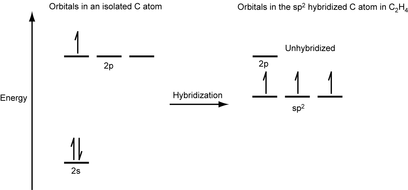
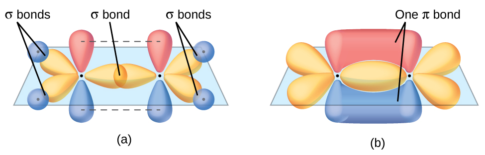
The three bonding regions form a trigonal planar electron region geometry. Thus we expect the σ bonds from each carbon atom are formed using a set of sp2 hybrid orbitals, resulting from hybridization of two of the 2p orbitals and the 2s orbital of carbon (Figure 26). These orbitals form two C–H single bonds and the σ bond in the C=C double bond (Figure 27). The π bond in the C=C double bond results from the overlap of the third (remaining) 2p orbital on each carbon atom that is not involved in hybridization. This unhybridized p orbital (lobes shown in red and blue in Figure 27) is perpendicular to the plane of the sp2 hybrid orbitals. Thus the unhybridized 2p orbitals overlap in a side-by-side fashion, above and below the internuclear axis (Figure 27) and form a single π bond.
In an ethene molecule, the four hydrogen atoms and the two carbon atoms are all in the same plane. If the two planes of sp2 hybrid orbitals are tilted relative to each other, the p orbitals would not be oriented to overlap efficiently to create the π bond. The planar configuration for the ethene molecule occurs because it is the most stable bonding arrangement. This is a significant difference between σ and π bonds; rotation around single (σ) bonds occurs easily because the end-to-end orbital overlap does not depend on the relative orientation of the orbitals on each atom in the bond. In other words, rotation around the internuclear axis does not change the extent to which the head-to-head σ bonding orbitals overlap because the bonding electron density is symmetric about the axis. Rotation about the internuclear axis is much more difficult for multiple bonds as it would drastically alter the off-axis overlap of the π bonding orbitals, essentially breaking the π bond.
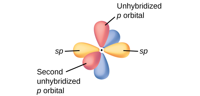
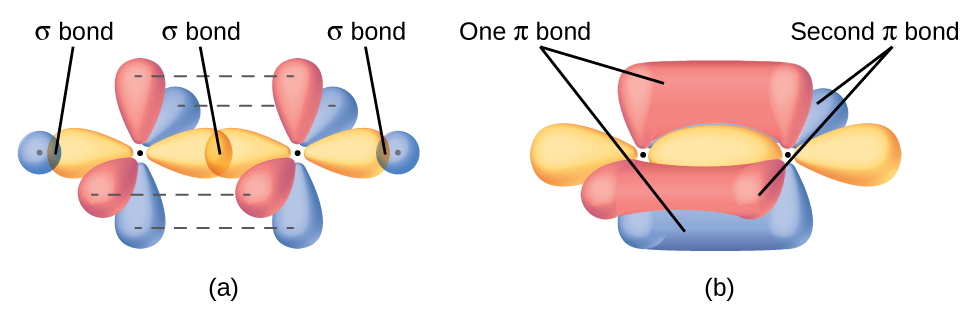
In molecules with sp hybrid orbitals, two unhybridized p orbitals remain on the atom (Figure 28). We find this situation in acetylene, H−C≡C−H, which is a linear molecule. The sp hybrid orbitals of the two carbon atoms overlap end to end to form a σ bond between the carbon atoms (Figure 29). The remaining sp orbitals form σ bonds with hydrogen atoms. The two unhybridized p orbitals per carbon are positioned such that they overlap side by side and, hence, form two π bonds. The two carbon atoms of acetylene are thus bound together by one σ bond and two π bonds, giving a triple bond.
Hybridization can model the basic bonding structure for many molecules. However, many molecules require another layer of complexity to produce a model that more accurately reflects experimental observations. One important example of this is resonance. Remember that resonance forms occur when various arrangements of π bonds are possible. Since the arrangement of π bonds involves only the unhybridized orbitals, resonance does not influence the assignment of hybridization.
For example, the molecule benzene has two resonance forms (Figure 30). We can use either of these forms to determine that each of the carbon atoms is bonded to three other atoms with no lone pairs, so the correct hybridization is sp2. The electrons in the unhybridized p orbitals form π bonds. Neither resonance structure completely describes the electrons in the π bonds. They are not located in one position or the other, but in reality are delocalized throughout the ring. Valence bond theory does not easily address delocalization.

Example 3
Assignment of Hybridization Involving Resonance
Some acid rain results from the reaction of sulfur dioxide with atmospheric water vapor, followed by the formation of sulfuric acid. Sulfur dioxide, SO2, is a major component of volcanic gases as well as a product of the combustion of sulfur-containing coal. What is the hybridization of the S atom in SO2?
Solution
The resonance structures of SO2 are

The sulfur atom is surrounded by two bonds and one lone pair of electrons in either resonance structure. Therefore, the electron region geometry is trigonal planar, and the hybridization of the sulfur atom is sp2.
Check Your Learning
Another acid in acid rain is nitric acid, HNO3, which is produced by the reaction of nitrogen dioxide, NO2, with atmospheric water vapor. What is the hybridization of the nitrogen atom in NO2? (Note: the lone electron on nitrogen occupies a hybridized orbital just as a lone pair would.)
Answer:
sp2
Key Concepts and Summary
In this section, we review many of the topics you are expected to be familiar with that are the foundation of organic chemistry. The first review topic is VSEPR Theory of two, three, and four electron regions. These electron region and molecular geometries enable us to predict molecular shape and bond angles. Using these molecular shapes, we can take a closer look at the electronegativity of the atoms within a molecule to predict if a molecule is polar. A molecule’s polarity determines many of its physical properties, like melting point.
After knowing both the molecular geometry and polarity, we can determine which intermolecular forces (IMF) each molecule interacts with. The stronger the IMF, the higher the melting and boiling points will be. Knowing which IMF exist within a chemical system will be extremely important for the rest of the semester! The weakest IMF are dispersion forces, which are present between all molecules with an electron, but are the only IMF between nonpolar molecules. The next strongest IMF are dipole-induced dipole forces. This IMF requires one molecule to be polar, while the other molecule is either polar or non-polar. The presence of the permanent dipole on one molecule induces a dipole (or a stronger/weaker dipole) in another molecule. The next IMF are dipole-dipole forces, which require both molecules to be polar. There is a special subset of dipole-dipole force called hydrogen bonding, which requires one molecule to have a hydrogen bonded to an F, O, or N and the other molecule to have a lone pair on F, O, or N. The strong but transient hydrogen bond forms between the hydrogen on on molecule and the lone pair on the other. IMF stronger than dipole-dipole require an ion to be present.
After we have reviewed molecular geometry and how that influences how molecules interact, it is important that we review the bonding between atoms within a molecule, first using valence bond theory. The bond between two atoms is created when a portion of orbitals on two adjacent atoms overlap and occupy the same region of space. The strength of this interaction is dependent on which orbitals are overlapping and if the interaction is head-to-head (a sigma interaction) or side-to-side (a pi interaction). Valence bond theory does not accurately predict the geometry of all molecules, so we instead look at a different corrective model called hybridization, where pure s or p orbitals are not overlapping between atoms, but rather a combination of these orbitals, known as sp, sp2 or sp3 orbitals (note: there are other hybrid orbitals, but these are the most common ones seen in organic chemistry). Using hybridization, we can also look at more complicated bonding interactions (like double and triple bonds) through the overlap of both hybrid orbitals as well as unhybridized p orbitals.
Glossary
- bond dipole moment
- the separation of charge that results when two atoms with differing electronegativites are bonded together, leaving a δ+ charge on the less electronegative atom and a δ- charge on the more electronegative atom
- dipole-dipole attraction
- the attractive force between two polar molecules, with the attraction between the partially positive end of one molecule and the partially negative end of another
- electron region geometry
- geometry based on all regions where electrons are located (bonds and lone electron pairs)
- hybridization
- a widely accepted model that uses quantum mechanics to mathematically combine valence orbitals and create new hybrid orbitals. This model explains the observed bond angles in water, and many other molecules
- hybrid orbitals
- the new orbitals created after hybridization
- hydrogen bonding
- a particularly strong type of dipole-dipole attraction, where the hydrogen of a molecule with F-H, O-H, or N-H is very strongly attracted to lone pairs on F, O or N in nearby molecules
- induced dipole
- a temporary dipole created by the presence of a dipole in a nearby atom or molecule
- instantaneous dipole
- a temporary dipole created by the constant motion of electrons in an atom or molecule
- intermolecular forces (IMF)
- the various forces of attraction that exist between atoms and/or molecules due to electrostatic properties
- molecular (overall) dipole moment
- the net charge separation in a molecule
- molecular geometry
- geometry only based on the location of atoms, not lone electron pairs
- node
- a plane with no probability of finding an electron
- nonpolar molecule
- a molecule without a dipole moment
- pi (π) bond
- a covalent bond where the overlap of electron density lies on opposite sides of the internuclear axis, or a side-to-side interaction
- polarizability
- the measure of how easy or difficult it is for another electrostatic charge (a nearby ion or molecule) to distort a molecule’s electron cloud
- polar molecule
- a molecule with a dipole moment
- sigma (σ) bond
- a covalent bond where the overlap of electron density is concentrated in the region along the internuclear axis, or a head-to-head interaction
- sp hybrid orbitals
- the hybrid orbitals that result from mixing one s orbital and one p orbital to produce two identical sp hybrid orbitals, leaving two unhybridized p orbitals
- sp2 hybrid orbitals
- the hybrid orbitals that result from mixing one s orbital and two p orbitals to produce three identical sp2 hybrid orbitals, leaving one unhybridized p orbital
- sp3 hybrid orbitals
- the hybrid orbitals that result from mixing one s orbital and all three p orbitals to produce four identical sp3 hybrid orbitals
- valence bond theory
- a theory that describes a covalent bond as the overlap of two half-filled atomic orbitals (each containing a single electron) that yield a pair of electrons shared between the two bonded atoms
- valence shell electron-pair repulsion theory (VSEPR theory)
- a theory to predict the molecular geometry, including approximate bond angles around a central atom, of a molecule from an examination of the number of bonds and lone electron pairs in its Lewis structure
- vector
- a quantity having both direction and magnitude
Chemistry End of Section Exercises
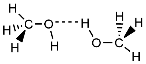
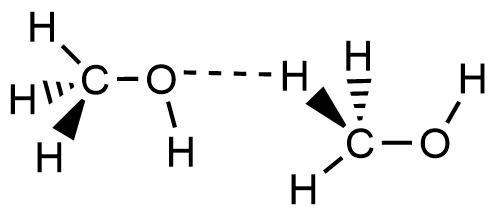
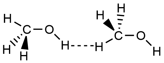
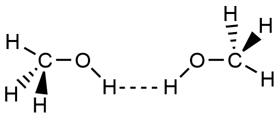
- Which of the following picture most accurately depicts hydrogen bonding in methanol?
Answers to Chemistry End of Section Exercises
- A
Please use this form to report any inconsistencies, errors, or other things you would like to change about this page. We appreciate your comments. 🙂
- Note that orbitals may sometimes be drawn in an elongated “balloon” shape rather than in a more realistic “plump” shape in order to make the geometry easier to visualize. ↵
